This Tip of the Month (TOTM) discusses how to increase production today, quickly, and for zero CAPEX. I’ll discuss the concepts, techniques, and where to look for and find opportunities, so we can answer the key question: “Are we getting the most from our asset?”
Many companies use benchmarking data shared anonymously with other participants in the survey. The problem is they will not have exactly the same assets. What’s being recommended here is that you benchmark you asset against physics and not others.
The good news is that no one can have better performance than the theoretical technical limit. If you determine your performance and compared it with a theoretical model / theoretical maximum and find a gap, then there’s an opportunity to improve.
BACKGROUND
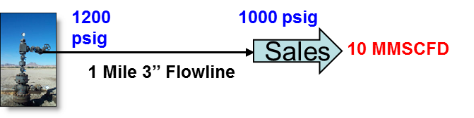
You have been asked by the Asset Manager to find opportunities to increase production. In this case the well is flowing at 1200 psig (8.3 MPag) downstream of a wide open choke into a 1 mile (1.6 km) 3inch (76 mm) flowline discharging into a sales line operating at 1000 psig (6.9 MPag), and flowing gas at 10 MMSCFD (0.28×10⁶ std m3/day).
KEY QUESTION – CASE 1
Is Today a good day? Are we getting the most from this asset?
Start by comparing the following:
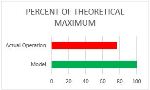
- What is the theoretical maximum given the current conditions – MODEL?
- What is the current operational performance – ACTUAL PERFORMANCE?
Figure 1 presents a bar chart for BENCHMARKING AGAINST PHYSICS.
The most common answer is that the well is online. We are selling gas, and the choke is wide open. There is no further investigation or action performed. This is because the gap cannot be seen without performing the engineering.
The answer from reading this TOTM should be:
- We have a process model that indicates that Benchmarking against PhysicsTM the flow line should be able to deliver 13 MMSCD (0.37×10⁶ std m3/day).
- You visit the field and verify the data. The gap is a 30% increase in production, see Figure 1.
- What’s causing this? Another block valve in the system? System Scale?
- How could you increase production quickly? Remove the entire choke body internals? Replace a small ported ball valve with a full ported valve? Recommend cleaning the line? Or simply opening a valve that is partially closed at the sales connection?
What’s the incremental value of 3 MMSCFD (0.085×10⁶ std m3/day) with $4/ MMBTU ($3.8/GJ) sales gas per year? $4.35 Million USD/year. Was that worth a field trip? Absolutely!
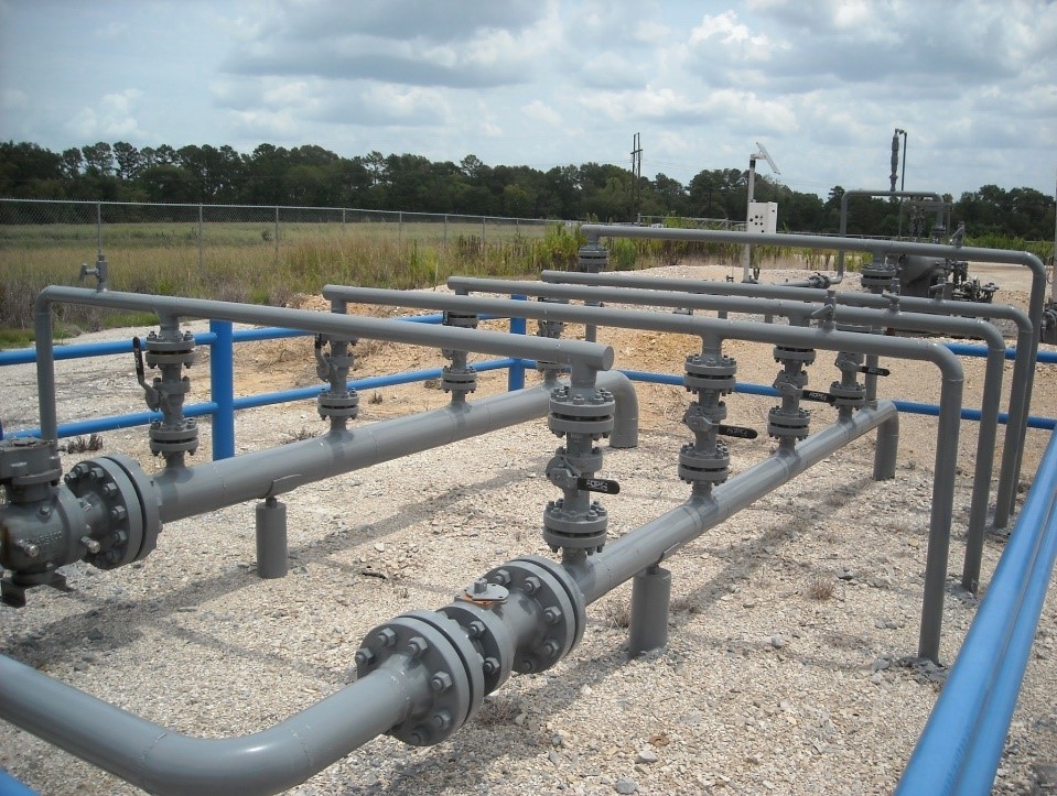
Figure 2. Flowline Manifold – Are these valves lined up properly? Could they be leaking?
In Figure 2, what are the implications of leaking manifold valves? Could HP (high pressure) wells be sending gas backwards into lower pressure wells? Are stronger wells backing out lower pressure wells to sales? Are a competitor’s higher pressure wells backing out our production?
KEY QUESTION – CASE 2
Is Anything wrong with our sale gas pipeline?
BACKGROUND
The pink points in Figure 3 are the gas sales in MMSCFD on the right axis, and the dark blue points are the pipeline differential pressure. The rate is decreasing over time and the pressure drop is decreasing over time.
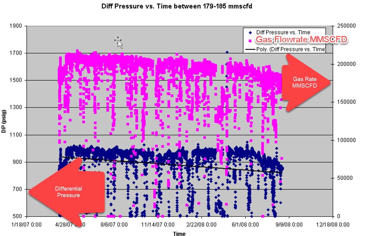
Figure 3. SCADA DATA for pipeline performance gas rate in MMSCFD and differential pressure over time
The pipeline is a 14 inch (356 mm) 60 mile (96 km) from a major offshore asset. If the gas pipeline becomes plugged, then the oil production and gas production needs to be shut down; approximately 100,000 bopd (15,900 m3/day) and 200 MMSCFD (5.65×10⁶ std m3/day) of gas. The operational data are presented in Table 1.
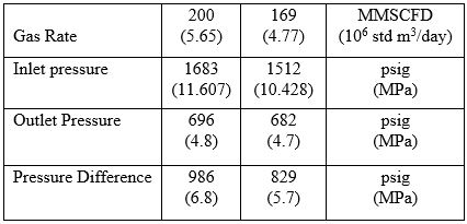
Table 1- Operational data performance
A UNISIM [1] Model shown in Figure 4 was completed to determine if the current performance matched the actual operational performance.
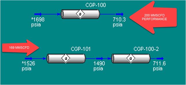
Figure 4 – UNISIM PIPELINE PERFORMANCE
The top pipeline simulation in Figure 4 matched the operating data performance at 200 MMSCFD (5.65×10⁶ std m3/day), however; the pipeline at the lower rate of 169 MMSCFD (4.77×10⁶ std m3/day) did not match the observed performance. In order to match the performance a choke 4 inches (102 mm) in diameter by 100 ft (31.1 m) was added to the 60 mile (96 km) 14 inch (356 mm) pipeline model.
The platform had been experiencing asphaltenes in its separators. They were lucky to have performed the engineering analysis, and have a scheduled shutdown to clean a section of the pipeline at the base of the sales gas riser. How are you monitoring your critical cash flow pipelines?
KEY QUESTION – CASE 3
How can we improve the performance of gas pipeline using SCADA data?
Here is another quick tip using SCADA Data and Excel.
From the GPSA Data Book [2] we know that gas flowrate (Q) is proportional to a constant times the square root of the static pressure (P1) times the differential pressure (ΔP).
![]()
So the trick is that if you construct a plot of C’ versus time… C’ is constant unless fouling has occurred. Fouling is difficult to find from just looking at data since it’s a chronic problem overtime, and not generally and acute one.
Figure 4 shows some SCADA Data using this technique. In order to scale the data, instead of C’ being plotted, the reciprocal of C’ squared was plotted to scale the plot. This still should be a constant over time, and you can see the inflection point on the red line on this two years of data.
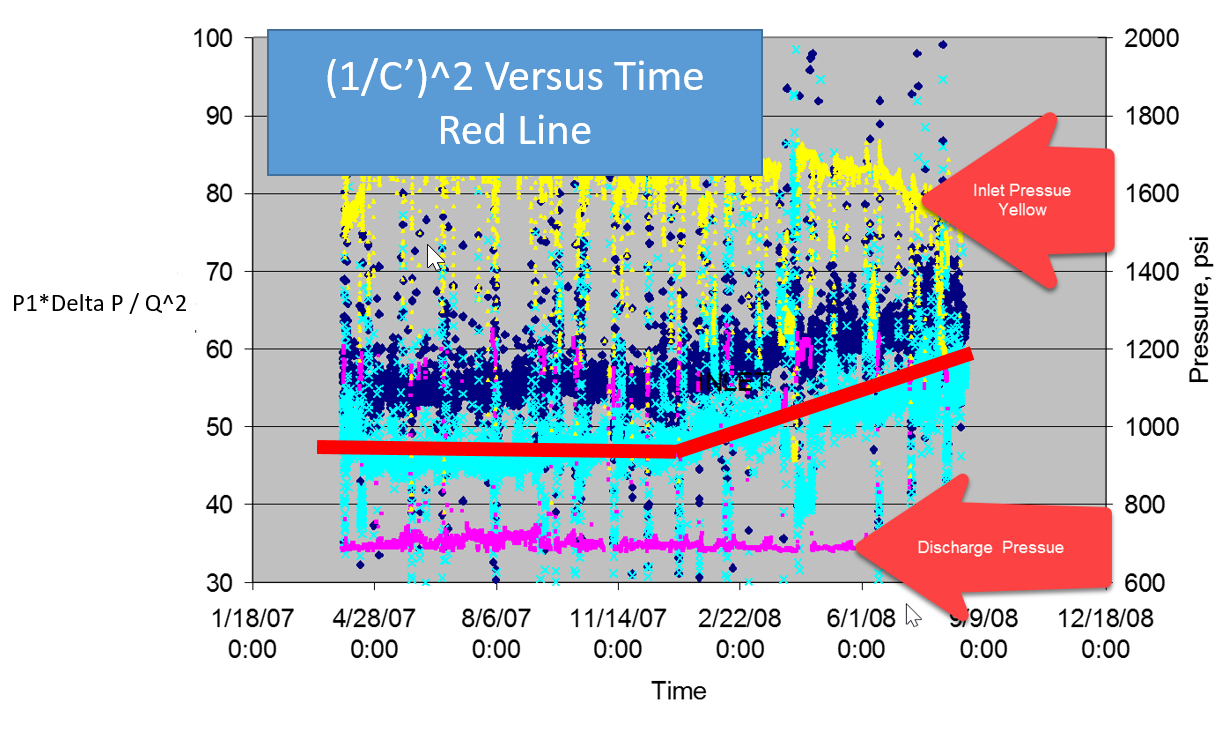
Figure 5. C’ Plot over time – Red line indicates a changing C’
Although this case reflected an asphaltene accumulation over time creating a localized plug. The unfavorable conditions would yield the same results as if it were a uniform scale along the entire pipeline length.
In upstream instances for subsurface models it’s difficult to see trends, because of the nature of the reservoir. We start off with high pressures, and flowrates, and these continually change over time. The compositions oil / gas / water and their relative proportions change as well over time. With all of these items changing overtime it’s sometimes difficult to detect small changes by simply looking at the data. As shown in the previous examples if you Benchmark Against PhysicsTM it becomes very clear what’s happening.
The last item we will add to the bar graph tool (Figure 6) is a bar for the original design capacity.
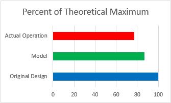
Figure 6. ACTUAL / MODEL / ORIGINAL DESIGN CONDITIONS
KEY QUESTION – CASE 4
How can we increase the Gas Plant Throughput to full capacity?
BACKGROUND
You get a call from one of your Gas Plants in Europe, and it’s having a problem. It used to operate at full capacity, but something has changed and the operators can’t get more than 50% capacity through the plant. The plant processes several Billion Standard Cubic Feet of gas per day, and at current rates will lose over a $1 Billion USD this year if it is not corrected.
You build a model to compare actual performance with theoretical, and you build the bar charts for major pieces of equipment throughout the gas plant. The plant is a straight refrigeration gas plant that has stabilization of recovered liquids. It’s been there for 20 years operating without a problem. It processes about one third of the gas coming into the country.
After looking at the model and the graphs it’s clear to you what the problem could be. I flew from Houston to London. Visited the plant. Assessed the situation, and made some setpoint changes with the operators which resolved the issue, and then flew back to Houston the next day.
Why did I take the time to visit the plant? Below is some sage advice from Norman Lieberman [3].
“The tech service engineers employed by my clients, who work with me on these jobs, always ask what special techniques I employ to solve these problems. The procedure I use is the same one I used 10 years ago:
- Discuss the problem with the shift operators.
- Personally collect field data and carefully observe the operation of the unit.
- Develop a theory as to the cause of the malfunction.
The error my clients often make is that they develop a theory, usually with process computer simulations, as to the cause of the malfunction. The theory is then reviewed with management and other technical personnel at a large meeting. If no one objects to the theory, it is accepted as the solution to the problem. Typically, no one at the meeting has discussed the problem or the solution with the shift operators, nor has anyone personally observed the process deficiency in the field. Finally, the intended solution is not put to a plant test to see if it is consistent with the problem. This approach to solving refinery process problems by the major oil companies often results in wasting capital resources and engineering man-hours.”
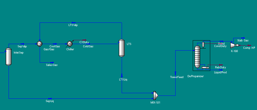
Figure 7. Gas Plant Process Flow Schematic UNISIM
The plant schematic is shown in Figure 7, and it’s a straight refrigeration plant with a low temperature separator and liquids stabilizer. The plant must meet a gas dewpoint specification and a maximum liquids vapor pressure – RVP (Reid Vapor Pressure). Figure 8. Presents Benchmarking Against Physics bar charts for the key components in this gas plant. Note that the RVP of 6 psi (42 kPa) is well below specified value of 12 psi (83 kPa) and the plant is operating at 50% of inlet capacity. The chiller is fully loaded. The stabilizer overhead compressor is fully loaded. They are meeting all specs.
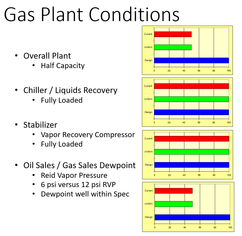
Figure 8
Figure 9 presents the gas plant schematic with bar charts for Benchmarking Against Physics.
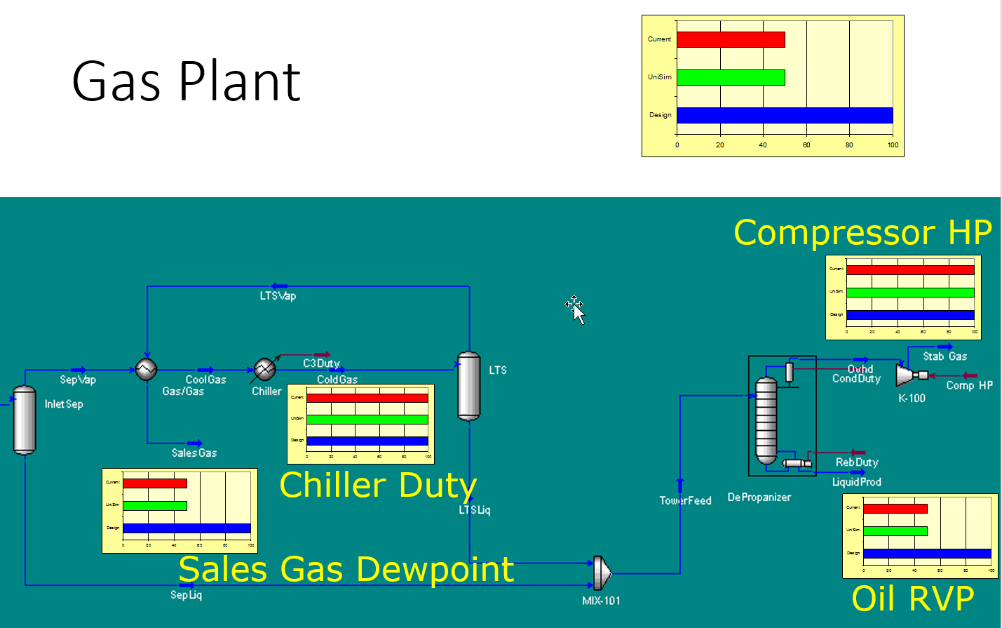 Figure 9
So what’s your conclusion? The stabilizer overhead compressor is a bottleneck and current operations are over stabilizing the liquids sending too much vapor overhead (Producing a 6 psi (41 kPa) RVP versus a specification of 12 psi (83 kPa)). If (they drop) the stabilizer bottoms temperature is reduced they will unload the stabilizer overhead compressor. If they still are exceeding the stabilizer overhead compressor, then they can reduce the liquids recovery by not chilling the gas as much. This will reduce the amount of liquid requiring stabilization. The next limit is the gas dewpoint spec, and they will need to chill the inlet gas sufficiently enough to meet the specification. Then they can begin increasing the inlet gas rate until they reach design maximum conditions.
Visiting the site, I found the plant operating as UNISIM predicted and the bar charts show. The operator’s mindset was that they needed to always chill the inlet gas to the maximum to make the company the most money. Then they backed themselves into a corner with the stabilizer operation. I went on rounds with them, and then suggest we try another approach and followed their management of change process to make setpoint changes. I explained the model results with them, and what we should expect to see as each change was slowly made. I have never shutdown a facility while making changes in 38 years because you always go slowly and are physically present to witness the cause and effects of changes. You never want to make a change and then hear the hiss of air leaving shutdown valve actuators and then have the lights go out. Going slowly builds the confidence of the operators in you and what you are doing. Bottom line is two temperature setpoints were adjusted within limits, and the plant was returned to full capacity in 8 hours. I then headed back to Houston for more adventures.
And as promised at the start of this TOTM…
“Increase Production Today, Quickly, and for Zero (increase in) CAPEX!”
Before you finish reading this article, please think about how to apply the concepts discussed, and TAKE ACTION in your work today. This type of work if fun and exciting…it translates directly to your company’s bottom line. Go forth, be safe, and make it a great day!
In the next TOTM I will present other places to look for optimization opportunities within your assets.
To learn more about similar cases and how to minimize operational problems, we suggest attending our G4 (Gas Conditioning and Processing), G5 (Advanced Applications in Gas Processing), PF3 (Concept Selection and Specification of Production Facilities in Field Development Projects), and PF49 (Troubleshooting Oil & Gas Processing Facilities) courses.
Reference:
- UNISIM Design R433, Honeywell International Inc., Calgary, Alberta, Canada, 2016
- Gas Processors Suppliers Association; “ENGINEERING DATA BOOK” 13th Edition; Tulsa, Oklahoma, USA, 2012.
- Norman P Lieberman, N P, “Troubleshooting Process Operations,” 4th Ed., PennWell, Tulsa, Oklahoma, 2009.

I enjoyed this – all what we are supposed to be about! I was taught by Crest Engineering – Original Outfit in London – We tackled North Sea Oil by the seat of our pants – Paper and Pen Engineering! No computers except the Mainframe Simulations I ran – 1977!
I like ‘Out of the Box’ Process Engineering.
Would like to keep in personal touch.
Best regards.
I have two questions – and need a broad brush idea.
Theoretically if we have Two Subsea Lines.
FULL CAPACITY – choked
20″ Slugging Wet Gas Line running 50 miles.
24″ Slugging Oil Line running the same 50 miles.
How much more Oil and how much more Gas flow can we get in each line if:
(1) Gas were to be running dry without slugging
– take an average terrain with slope, going up, to Shore
(2) Same goes for Oil.
(3) If we could get Stabilized NGL at source.
Thank you in advance.