Category: Pipeline

  • Low Pressure Versus High Pressure Dense Phase Natural Gas Pipeline Transportation

    Dense phase is a favorable condition for transporting carbon dioxide (CO2) and natural gas as well as carbon dioxide injection into crude oil reservoir for enhanced oil recovery. Pipelines have been built to transport CO2 and natural gas [1] in the dense phase region due to its higher density, and this also provides the added benefit of no liquids formation in the pipeline.

    Recently (January through April 2012 TOTMs) we discussed several aspects of transportation of carbon dioxide (CO2) in the dense phase. We illustrated how thermophysical properties change in the dense phase and their impacts on pressure drop calculations. The pressure drop calculation utilizing the liquid phase and vapor phase equations were compared. In the August 2012 Tip of The Month (TOTM) [2], we studied transportation of rich natural gas in the dense phase region and compared the results with the case of transporting the same gas using a two phase (gas-liquid) option. Our study highlighted the pros and cons of dense phase transportation.

    In this TOTM, we will study the low pressure versus high pressure (dense phase) pipeline transportation of a lean natural gas. The application of dense phase in the oil and gas industry will be discussed briefly.

    Case Study:

    For the purpose of illustration, we will consider transporting a natural gas mixture with composition and conditions presented in Table 1. For simplicity, the calculations and subsequent discussion will be done on the dry basis. The feed gas dew point was reduced to -40 ˚F (-40 ˚C) by passing it through a mechanical refrigeration dew point control plant. Figure 1 presents the phase envelopes for the feed and lean (pipeline) gases. The composition and conditions of the lean gas are also presented in Table 1. The 1000 miles (1609 km) long pipeline with a  diameters of 42 inches (1067 mm) has been considered. A simplistic Process Flow Diagram (PFD) is shown in Figure 2. The following assumptions and correlations are/used:

    1. Dry basis, ignoring water.
    2. C7+ considered as nC8.
    3. Steady state
    4. Delivery pressure is 615 Psia (4.24 MPa).
    5. Pressure drop in each heat exchanger is 5 psi (0.035 MPa).
    6. No pressure drop in scrubbers and separators.
    7. Horizontal pipeline, no elevation change.
    8. Inside surface absolute roughness is 0.0018 in (0.046 mm).
    9. Single Phase Friction Factor: Colebrook
    10. For calculation purpose, each line segment was divided into 10 sub segments.
    11. Overall Heat Transfer Coefficient: 0.25 Btu/hr-ft2-˚F (1.42 W/m2-˚C).
    12. Simulation software: ProMax [3]
    13. Equation of State: Soave-Redlich-Kwong (SRK).

    Table 1. Composition and conditions of the feed gas and lean gas


    Figure 1. Phase envelopes for the feed (rich) and pipeline (lean) gas


    Three cases for transportation of this natural gas are considered and each is explained briefly in the proceeding section. Figure 2 presents the PFDs for Cases A and B. Case C PFD is similar to Case B with 2 more pipeline segments, compressors and coolers. Figure 3 illustrates the pipeline systems in a block diagram.  The number of pipeline segments, segment length, and inlet pressure of each segment for the three cases are presented in Table 2 in the field (FPS, foot, pound and second) and SI (System International) sets of units.

    Figure 2. Process flow diagrams (PFD) for Cases A and B (Case C is similar to Case B)


    Figure 3. Pipeline Block Diagrams for Cases A, B, and C

    Table 2. Pipeline specifications for the three cases


    Case A: High Pressure (Dense Phase)

    After passing through the first stage scrubber, the lean gas enters the first stage of compressor where its pressure is raised to 1407 psia (9.703 MPa), then it is cooled to 100 ˚F (37.8 ˚C) and compressed further in the second stage to 3220 Psia (22.2 MPa). The high pressure compressed gas is cooled back to 100 ˚F (37.8 ˚C) and then passed through a separator before entering the long pipeline (See Case A in Figure 2).


    Case B: Intermediate Pressure

    The process flow diagram (PFD) for this case is also shown in Figure 2. In this case, the pipeline is divided into three 333.3-mile (536.2 km) pipelines with one lead compressor station and two intermediate compressor stations. In each station, the pressure is raised from 615 Psia to 1966 Psia (4.24 to 13.56 MPa) in one stage and then cooled to 100 ˚F (37.8 ˚C), passed through a separator before entering the downstream pipeline segment.


    Case C: Low Pressure

    This case is similar to Case B except the pipeline is divided into five 200-mile (322 km) pipeline segments with one lead compressor station and 4 intermediate compressor stations. In each station, the pressure is raised from 615 Psia to 1600 Psia (4.24 to 11.03 MPa) in one stage and then cooled to 100 ˚F (37.8 ˚C), passed through a separator before entering the downstream pipeline segment.


    Simulation Results and Discussions:

    The PFDs for the three cases are simulated using ProMax [3]. To improve the accuracy and to take care of variations of physical properties of gas, each pipeline segment length was divided into 10 sub segments. For Case A in which pipeline segment was considerably longer, we tried 50 and 100 sub segments and no change in the outlet pressure and temperature was observed. Table 3 presents a summary of simulation results for the three cases in the field and SI system of units. As can be seen in this table, Case A requires the least total compression power and heat duty requirements. The power reduction for Case A is about 51%  compare to Case B and 63% compare to Case C. These reductions in power and heat duty requirements are considerable.  Similarly, the heat duty reduction for Case A is about 39% compared to Case B and 50 % compare to Case C, respectively.

    Table 3. Summary of computer simulation results for the three cases.

    Figure 4 presents the phase envelope, the required compression and cooling stages and pipeline pressure-temperature profile for Case A. This figure shows that the pipeline outlet condition ends up to the right of the dew point curve with the gas remaining as single phase.
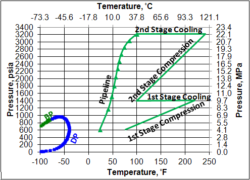
    Figure 4. Phase envelope, compression and cooling stages and pipeline pressure-temperature profile (ID=42 in = 1067 mm)

    Pipeline wall thickness is an important economic factor. The wall thickness, t, for the three cases was calculated by:

    Where,

    P is maximum allowable operating pressure, here set to 1.1 times the inlet pressure,

    OD is outside diameter,

    E is joint efficiency (assumed to be 1),

    f1 is wall thickness tolerance (assumed to be 1.0),

    f2 is design factor, 0.4 to 0.72  and here set  to be 0.72 for remote area),

    σ is the pipe material yield stress (assumed pipe material grade X65 to be 65,000 psi or

    448.2 MPa), and

    CA is the corrosion allowance (assumed to be 0 in or 0 mm, for dry gas).


    Figure 5 presents the calculated wall thickness as a function of the inlet pressure (for the three cases). Notice Case A requires the largest and Case C requires the smallest wall thickness.

    Variation of density, viscosity, velocity, pressure, and temperature along the pipeline are shown in Figures 6 through 10 for Cases A and B.

    Conclusions:

    We have studied transportation of natural gas in the dense phase region (high pressure) and compared the results with the cases of transporting the same gas using intermediate and low pressures. Our study highlights the following features:

    1. If the gas at the source is not at high enough pressure, considerable compression power and cooling duty may be required if the decision is to use the dense phase.
    2. For the dense phase – Case A, (high pressure), higher wall thickness is required.
    3. For the dense phase – Case A, lower compressor power and heat duty are required.
    4. For the dense phase – Case A, the friction pressure drop / mile is lower .
    5. For the dense phase – Case A and the same diameter, on the average the velocity is lower compared to lower pressure gas transportation.

    Other logical results can be stated as well including:

    1. Composition of the gas plays an important role.
    2. Pipeline elevation profile and distance may be  important factors at the higher operating pressures.
    3. A detailed economic analysis in terms of CAPEX and OPEX should be made for a sound comparison.

    In a future Tip of the Month, we will consider the design and order of magnitude costs impacts when constructing each of these three cases, first onshore then offshore.

    To learn more about similar cases and how to minimize operational problems, we suggest attending our G40 (Process/Facility Fundamentals), G4 (Gas Conditioning and Processing), G5 (Gas Conditioning and Processing-Special), P81 (CO2 Surface Facilities), PF4 (Oil Production and Processing Facilities), and PL 4 (Fundamentals of Onshore and Offshore Pipeline Systems) courses.

    John M. Campbell Consulting (JMCC) offers consulting expertise on this subject and many others. For more information about the services JMCC provides, visit our website at www.jmcampbellconsulting.com, or email your consulting needs to consulting@jmcampbell.com.

    By: Mahmood Moshfeghian and David Hairston

    References:

    1. Beaubouef, B., “Nord stream completes the world’s longest subsea pipeline,” Offshore, P30, December 2011.
    2. http://www.jmcampbell.com/tip-of-the-month/
    3. ProMax 3.2, Bryan Research and Engineering, Inc., Bryan, Texas, 2012.


    Figure 5. Variation of wall thickness with pipeline inlet pressure

    Figure 6. Variation of gas density in the pipeline (Cases A and B)

    Figure 7. Variation of gas viscosity in the pipeline (Cases A and B)

    Figure 8. Variation of gas velocity in the pipeline (Cases A and B)

    Figure 9. Variation of pressure in the pipeline (Cases A and B)

    Figure 10. Variation of temperature in the pipeline (Cases A and B)

  • Considering the effect of crude oil viscosity on pumping requirements

    In the August 2009 Tip of the Month (TOTM), it was shown that pumping power requirement varies as the crude oil °API changes. Increasing °API or line average temperature reduces the crude oil viscosity. The viscosity reduction caused higher Reynolds number, lower friction factor and in effect lowered pumping power requirements. Since the objective of the August 2009 TOTM was to study the effect °API and the line average temperature have on the pumping power requirement, the effect of crude oil viscosity on pump performance was ignored and in the course of calculation a constant pump efficiency of  =0.75 was used for all cases. In this TOTM, we will consider the crude oil viscosity effect on a selected pump performance. The Hydraulic Institute Standards [1] procedures and the guideline presented in the August 2006 TOTM written by Honeywell were applied to correct the pump efficiency.

    As in the August 2009 TOTM, we will study crude oil °API and the pipeline average temperature and how these effect the pumping requirement. For a case study, we will consider a 160.9 km (100 miles) pipeline with an outside diameter of 406.4 mm (16 in) carrying crude oil with a flow rate of 0.313 m3/s or 1,126 m3/h (170,000 bbl/day or 4958 GPM). The pipeline design pressure is 8.963 MPa (1300 psia) with a maximum operating pressure of 8.067 MPa (1170 psia). The wall thickness was estimated to be 6.12 mm (0.24 in). The wall roughness is 51 microns (0.002 in) or a relative roughness (e/D) of 0.00013. The procedures outlined in the March 2009 TOTM were used to calculate the line pressure drop due to friction. Then corrected pumping efficiency was used to calculate the required pumping power. Since the objective was to study the effect °API and the line average temperature have on the pumping power requirement, we will ignore elevation change. The change in pumping power requirements due to changes in crude oil °API and line average temperature for this case study will be demonstrated.

    Viscosity Effect on Centrifugal Pump Performance
    There are several papers investigating and presenting procedures for correcting centrifugal pump curves [2-3].  According to Turzo et al. [2], three models are available for correcting performance curves: Hydraulic Institute, Stepanoff, and Paciga.  Turzo et al. [2] also presented a computer applications for correcting pump curves for viscosity effect. In this review, the Hydraulic Institute [1], HI, procedure was applied and is described briefly here.

    HI uses a performance factor, called Parameter B which includes terms for viscosity, speed, flow rate and total head. The method uses a new basis for determining the correction factors CH, CQ, and C.  The basic equation for Parameter B is given as Equation 1.

    Equation 1

    B = Performance factor
    K = 16.5 for SI units
    = 26.5 for USCS (FPS)
    Nuvis = Viscous fluid Kinematic viscosity – cSt
    HBEP-W = Water head per stage at BEP – m (ft)
    QBEP-W = Water flow rate at BEP – m3/h (gpm)
    N = Pump shaft speed – rpm

    Correction factors are applied to capacity (CQ), head (CH), and efficiency (CNu). Calculation of these Correction Factors is dependent on the calculated value of Parameter B. For the cases considered in this study, the B values were less than 1; therefore, based on the HI guideline, the correction factors for head and capacity were set equal to 1 and the correction factor for efficiency, CNu, was calculated by Equation 2.

    Equation 2

    Nu BEP-W = Pump efficiency at BEP
    Vw = Water kinematic viscosity – cSt

    Figures 1 and 2 present the water-based pump curves used in this study. For computer calculations, these two curves were fitted to polynomials of degrees 3 and 2 for head vs capacity and efficiency vs capacity, respectively.

    Equations

    In Equations 3 and 4, H is in m (ft) and Q is in m3/h (GPM). For this pump:

    HBEP-W=323m=1060ft,       QBEP-W =1726 m3/h= 7600 GPM, N=1780 rpm, and NuBEP-W =83.4.

    Figure 1

    Case Study 1: Effect of Line Average Temperature (Seasonal Variation)
    To study the effect of the line average temperature on the pumping power requirement, an in house computer program called OP&P (Oil Production and Processing) was used to perform the calculations outlined in the March 2009 TOTM. For a 35 °API crude oil in the pipeline described the required pumping power was calculated for line average temperature ranging 21.1 to 37.8 °C (70 to 100 °F). For each case, the parameter B was calculated by Equation 1 and since its value was less than 1, the efficiency correction factor was calculated by Equation 2. Then, the pump efficiency calculated by Equation 4 was multiplied by the correction factor for the subsequent calculations. The corrected efficiency ranged from 0.70 to 0.72. The required pumping power was compared with an arbitrary base case (85 °F or 29.4 °C and constant Nu = 0.75) and the percentage change in the pumping power requirement was calculated. Figure 3 presents the percent change in power requirement as a function of line average temperature. There is about 5% change (for constant Nu=0.75) and more than 8% change (for corrected efficiency) in the pumping power requirement for the temperature range considered.

    Figure 2

    Note that as the line average temperature increases the power requirement decreases. This can be explained by referring to Figure 4 in which the oil viscosity decreases as the temperature increases. Lower viscosity results in higher Reynolds (i.e. Reynolds number Equation which is the ratio of inertia force to viscous force); therefore, the friction factor decreases (refer to the Moody friction factor diagram in the March 2009 TOTM).

    Figure 3

    Case Study 2: Effect of Variation of Crude Oil °API
    In this case, the effect of crude oil °API on the total pump power requirement for three different line average temperatures was studied. For each line average temperature, the crude oil °API was varied from 30 to 40 and the total pumping power requirement was calculated and compared to the base case (35 °API and average line temperature of 29.4°C=85°F).

    For each case the percent change in total power requirement was calculated and is presented in Figure 5. As shown, when °API increases the total power requirement decreases. This also can be explained by referring to Figure 4 in which the crude oil viscosity decreases as ° API increases. The effect of viscosity is more pronounced at lower line average temperature (i.e. 21.1 °C or 70°F). Figure 5 also indicates that there is about 30 % change in total power requirement as °API varies from 30 to 40 °API. This is a significant variation and suggests that it should be considered during design of crude oil pipelines.

    Discussion and Conclusions
    The analysis of Figures 3 and 5 indicates that for the oil pipeline, the pumping power requirement varies as the crude oil °API changes. Increasing °API or line average temperature reduces the crude oil viscosity (see Figure 4). The reduction of viscosity results in higher a Reynolds number, lower friction factor and in effect lowers pumping power requirements.

    For the cases studied in this TOTM, the effect of crude oil viscosity on the performance of pump was considered. It was found that no correction was required for the capacity and head but a correction factor in the range of 0.95 to 0.98 was required to adjust the pump efficiency for crude oil applications.

    Figure 4

    A sound pipeline design should consider expected variations in crude oil °API and the line average temperature. In addition, the pump performance curves should be corrected for the effect of viscosity.

    To learn more about similar cases and how to minimize operational problems, we suggest attending our ME44 (Overview of Pumps and Compressors in Oil and Gas Facilities)ME46 (Compressor Systems – Mechanical Design and Specification)PL4 (Fundamental Pipeline Engineering)G40 (Process/Facility Fundamentals)G4 (Gas Conditioning and Processing), and PF4 (Oil Production and Processing Facilities) courses.

    By: Dr. Mahmood Moshfeghian

    Figure 5

    References:

    • ANSI HI 9.6.7-2004, “Effects of Liquid Viscosity on Rotodynamic (Centrifugal and Vertical) Pump Performance”, 2004.
    • Turzo, Z.; Takacs, G. and Zsuga, J., “Equations Correct Centrifugal Pump Curves for Viscosity,” Oil & Gas J., pp. 57-61, May 2000.
    • Karassik, I.J., “Centrifugal Pumps and System Hydraulics,” Chem. Engr. J., pp.84-106, Oct. 4, 1982
  • How sensitive are crude oil pumping requirements to viscosity?

    During the life cycle of a crude oil pipeline the properties of transported oil change, because in gathering systems the produced oils come from different wells. New wells may be added or some wells may go out of production for maintenance and repair. Production rates during the life of wells vary, too. In addition the properties of crude oil change during production. Due to seasonal variation, the average line temperature may also change. As it is shown in the proceeding sections, viscosity of crude oil is a strong function of API gravity and temperature.

    In the March 2009 tip of the month (TOTM), procedures for calculation of friction losses in oil and gas pipelines were presented. The sensitivity of friction pressure drop with the wall roughness factor was also demonstrated.

    In this TOTM, we will study crude oil °API and the pipeline average temperature and how they effect the pumping requirement. For a case study, we will consider a 160.9 km (100 miles) pipeline with an outside diameter of 406.4 mm (16 in) carrying crude oil with a flow rate of 0.313 m3/s (170,000 bbl/day). The pipeline design pressure is 8.963 MPa (1300 psia) with a maximum operating pressure of 8.067 MPa (1170 psia). The wall thickness was estimated to be 6.12 mm (0.24 in). The wall roughness is 51 microns (0.002 in) or a relative roughness (e/D) of 0.00013. The procedures outlined in the March 2009 TOTM were used to calculate the line pressure drop due to friction. Then assuming 75 % pumping efficiency, the required pumping power was calculated. Since the objective was to study the effect °API and the line average temperature have on the pumping power requirement, we will ignore elevation change. The change in pumping power requirements due to changes in crude oil °API and line average temperature for this case study will be demonstrated.

    Case Study 1: Effect of Line Average Temperature (Seasonal Variation)

    To study the effect of the line average temperature on the pumping power requirement, an in house computer program called OP&P (Oil Production and Processing) was used to perform the calculations as outlined in the March 2009 TOTM. For a 35 °API crude oil in the pipeline described in the preceding section, the required pumping power was calculated for the line average temperature ranging from 21.1 to 37.8 °C (70 to 100 °F). For each case, the required pumping power was compared with an arbitrary base case (85 °F or 29.4 °C) and the percentage change in the pumping power requirement was calculated, accordingly. Figure 1 presents the percent change in power requirement as a function of line average temperature. There is about 5% change in the pumping power requirement for the temperature range considered.

    Figure 1

    Note as the line average temperature increases, the power requirement decreases. This can be explained by referring to Figure 2 in which the oil viscosity decreases as the temperature increases. Lower viscosity results in higher Reynolds (i.e. Reynolds number Equation is the ratio of inertia force to viscous force); therefore, the friction factor decreases (refer to the Moody friction factor diagram in the March 2009 TOTM).

    Case Study 2: Effect of Variation of Crude Oil API
    In this case, the effect of crude oil °API on the total pump power requirement for three different line average temperatures was studied. For each line average temperature, the crude oil °API was varied from 30 to 40 and the total pumping power requirement was calculated and compared to the base case (35 °API and average line temperature of 29.4°C=85°F).

    Figure 2

    Figure 3

    For each case the percent change in total power requirement was calculated and is presented in Figure 3. As shown in this figure, when °API increases the total power requirement decreases. This also can be explained by referring to Figure 2 in which the crude oil viscosity decreases as ° API increases. The effect of viscosity is more pronounced at lower line average temperature (i.e. 21.1 °C or 70°F). Figure 3 also indicates that there is about 25 % change in total power requirement as °API varies from 30 to 40 °API. This is a big change and should be considered during design of crude oil pipelines.

    Discussion and Conclusions
    The analysis of Figure1-3 indicates that for the oil pipeline, the pumping power requirement varies as the crude oil °API changes. Increasing °API or line average temperature reduces the crude oil viscosity (see Figure 2). The reduction of viscosity results in higher Reynolds number, lower friction factor and in effect lower pumping power requirements.

    In practical situations, an originating station takes crude out of storage and the midline stations taking suction from the upstream section of pipeline. In some parts of the world, the suction temperature to the originating pumps is +38 °C (+100 °F) but the temperature to the midline station is ground temperature (this assumes a buried line below the frost line) approximately 18 °C (65 °F). The originating station will always be more affected by temperature because storage will follow ambient – whereas the midline station will operate at notionally constant temperature +/- 5.5 °C (+/- 10 °F) in the lower 9 °C (48 °F). For the case studied in this TOTM, the number of pumping stations varied from 2.5 to 3.2.
    In light of the above discussion, a sound pipeline design should consider expected variation in crude oil °API and the line average temperature.

    To learn more about similar cases and how to minimize operational problems, we suggest attending our ME44 (Overview of Pumps and Compressors in Oil and Gas Facilities), ME46 (Compressor Systems – Mechanical Design and Specification)PL4 (Fundamental Pipeline Engineering)G40 (Process/Facility Fundamentals)G4 (Gas Conditioning and Processing), and PF4 (Oil Production and Processing Facilities) courses.

    By: Dr. Mahmood Moshfeghian

  • The Sensitivity of k-Values on Compressor Performance

    One of the most important physical properties of a gas is the ratio of specific heats.  It is used in the design and evaluation of many processes.  For compressors, it is used in the design of components and determination of the overall performance of the machine.  Engineers are frequently asked to evaluate a compressor performance utilizing traditional equations of head, power and discharge temperature.  While these simplified equations may not give exact results, they give useful information needed to troubleshoot a machine, predict operating conditions, or a long-term trend analysis.  The accuracy of the performance information will depend on the proper selection of the ratio of specific heats.  This Tip of the Month (TOTM) will investigate the application of the ratio of specific heats to compressors, its sensitivity to the determination of machine performance and give recommendations for improved accuracy.

    Background of k-value

    The ratio of specific heats is a physical property of pure gases and gas mixtures and is known by many other names including: adiabatic exponent, isentropic exponent, and k-value.   It is used to define basic gas processes including adiabatic and polytropic compression.  It also appears in many of the traditional equations commonly used to determine a compressor head, gas discharge temperature, gas power, and polytropic exponent.  The k-value also influences the operating speed of a compressor, but we will simplify the present analysis by deleting speed from our evaluation.  The following commonly used compressor performance equations show how the k-value is utilized in the design and evaluation of compressors.

    Equations

    Note:    The actual Z-value will vary from the suction to discharge conditions.  ZS is sometimes replaced with ZAVE to approximate the variations in compressibility value [1, 5]. See the nomenclature at the end of this TOTM.

    The above equations are written in terms of the adiabatic process with the exception of Equation 5, which refers to the polytropic process.  Both compression processes are similar and will give the same actual results.  The adiabatic and polytropic methods are extensively used by manufacturers to design compressors, and make use of k-values to calculate their performance.  However, as will be seen, the effect of the k-value and the calculated results will influence both compression processes alike.  For simplicity, this Tip of the Month will use the adiabatic process.
    It can be seen from Equations 1-5 that the k-value has an effect on a compressor head, temperature, power, and polytropic exponent.  In order to determine how small changes in the k-value can influence a compressor performance, let us first define the k-value of a pure gas.  The thermodynamic definition of a gas k-value is given by Equation 6.  It shows the relationship to the specific heat at constant volume, CV and specific heat at constant pressure, CP.  Both values vary with temperature and pressure.

    Equation

    For a pure gas there are many references that give CP and CV values at various conditions.  One useful source is National Institute of Standards and Technology.  Their website is http://webbook.nist.gov/chemistry/fluid/

    The method of determining the k-value for gas mixtures is more complex.  The major difference is that a gas mixture does not behave as any one of its components but as an “equivalent” gas.  Therefore, to determine the k-value of the mixture, we must know the mole fraction of each component, Yi and the molar specific heat at constant pressure for each component, M CPi.   Equation 7 can be used to determine the k-value of an ideal gas mixture [1, 5].  Real gases may deviate from the calculated value.

    Equation

    While Equations 1-7 are applicable for manual calculations methods, it is important to note that process simulation packages determine the compressor head and discharge temperature utilizing equations of state.  The results are the same but the methods are very different.

    K-value Sensitivity Analysis

    In the compression process the temperature and pressure of the process gas both increase.  Not knowing what k-value to select for evaluating the compression process can lead to errors.  For example, a typical propane compressor may have a k-value at suction conditions of 1.195.  At the compressor discharge conditions the k-value is 1.254.  The difference in the two values varies by 4.94 percent and can have a significant influence in the performance evaluation.  The following example illustrates how minor changes in the k-value can influence the calculated compressor head, temperature, power and the polytropic coefficient.

    Example 1: A natural gas compressor is operating at the conditions given below.  Only the k-value is varied from 1.20 to 1.28, all other given parameters remain constant.   Figure 1 illustrates how the “apparent” performance of a compressor can change by varying the k-value.

    Figure 1

    It can be seen from Figure 1 that the discharge temperature deviated over 18.8 percent by only changing the k-value by 6.7 percent.  In this case the k-value varied from a value of 1.20 to 1.28; which is the typical range for natural gas.  Similarly, the power changed by 2.5 percent, polytropic exponent by 9.5 percent, and adiabatic head by 2.5 percent for the same variation of the k-value.  The changes in compressor performance described in Figure 1 can be much larger depending on the gas composition and the operating temperature and pressure.

    Corrected k-Value Recommendations

    The k-value sensitivity for a single-stage machine is not nearly the problem as a multi-stage compressor.  For a single-stage machine, the pressure ratio is typically lower and the temperature and pressure changes are less.  As a result the changes in k-value are not as great and accurate results can be obtained by approximating the k-value at the suction conditions.  However, for multi-stage machines, where the pressure and temperature ratios are higher, the k-value sensitivity is more of a factor in evaluating compressor performance. Most compressor manufacturers calculate the k-value for each stage of compression and avoid errors introduced by utilizing an overall k-value. Without their software, we are left with a corrected k-value by empirical methods.

    There are many useful approximations that will correct for changes in the k-value as the process gas passes through the compressor.  Normally the k-value will decrease during compression but not always.  Utilizing the suction conditions to estimate the k-value will generally give higher values of temperature, heat, and power.  The polytropic exponent generally decreases as the adiabatic exponent decreases.  To avoid potential discrepancies, a k-value correct may be warranted.  The following are six methods of determining the corrected k-value commonly used in industry.

    1. At TS and PS:  This method determines the k-value at suction conditions and is useful for single stage compressors or applications where there is little change in the k-value.  The k-value is easy to determine and tends to overestimate results, especially if the temperature and pressure do not change significantly.  For greater values of RP the results may become so conservative they become useless.kks at suction conditions
    2. At TD and PD:  This method determines the k-value at discharge conditions.  The k-value is less conservative and tends to underestimate results.  The k-value may be difficult to determine, especially if the discharge temperature is unknown.    For gases with highly variable k-values, an iterative solution may be required to estimate the discharge temperature and corrected k-value.kkD at discharge conditions
    3. At TAVE and PSTD [5]:  This method utilizes the average operating temperature at standard pressure and determines the k-value.  Numerous reference books propose this method.  Errors are introduced because the k-value at standard pressure may not accurately represent values at the operating pressure.k = at average operating temperature and standard pressure
    4. At TAVE and PAVE:  This method utilizes the k-value at the average operating temperature and pressure.k = at average operating temperature and pressure
    5. Average value [1, 3]:  This empirical method takes the average k-value at compressor inlet conditions and outlet conditions.  Utilizing the average k-value will result in performance values that are closer to the actual performance of the compressor.Equation
    6. Weighted average value [4]: This empirical method takes the weighted average of the suction, mid-point and discharge conditions.  Note that the mid-pressure is determined by equivalent pressure ratios, Equation.  The mid-temperature is estimated from the mid-pressure.  This method considers the staged k-value to change with diverging isentropic and pressure lines shown on a Mollier chart.
    Equation

    Example 2 illustrates the various methods used to determine corrected k-values given above.  It also compares the range of the resulting values.

    Example 2: A propane compressor is operating at the given conditions shown below.  Table 1 lists the k-values attributed to various operating and reference conditions [6].

    Table 1

    Summary

    This Tip of the Month has defined the physical property of process gases called the k-value or ratio of specific heats.  It has shown that small changes in the k-value can have a significant effect on the calculated values of head, power, gas discharge temperature, and polytropic exponent.  Recommendations were also given to improve the accuracy by utilizing different k-value methods.

    To learn more about similar cases, we suggest attending our ME44 (Overview of Pumps and Compressors in Oil and Gas Facilities)ME46 (Compressor Systems – Mechanical Design and Specification)PL4 (Fundamental Pipeline Engineering)G40 (Process/Facility Fundamentals)G4 (Gas Conditioning and Processing), and PF4 (Oil Production and Processing Facilities) courses.

    By: Joe Honeywell

    Nomenclature

    References

    1. Ronald P Lapina, Estimating Centrifugal Compressor Performance, Vol. 1, Gulf Publishing, 1982.
    2. John M. Campbell, Gas Conditioning and Processing, Vol. 2, John M. Campbell & Co., 8th Edition.
    3. Elliott Compressor Refresher Course,
    4. John M. Schultz, “The Polytropic Analysis of Centrifugal Compressors”, Journal of Engineering for Power, January 1962.
    5. Gas Processor Suppliers Association, Engineering Data Book, Section 13, 2004
    6. National Institute of Standards and Technology, Web Site for Properties of Propane, Fluid Data.
    7. ASME PTC10-1997, Performance Test Codes, “Compressors and Exhausters”, R2003
  • Quick Determination of the Methanol Injection Rate for Natural-Gas Hydrate Inhibition

    The formation of hydrates in processing facilities and pipelines has been a problem to the natural gas industry. Whether the problem occurs in transportation or processing, hydrate formation can cause shutdowns and even destruction of valuable equipment. Because of these devastating and often costly consequences of hydrate formation, methods have been applied to prevent hydrate development in gas streams. The conditions that tend to promote hydrate formation include: low temperature, high pressure, and a gas at or below its water dew point temperature with “free” water present.  The formation of hydrates can be prevented by using any of the following techniques; (a) adjusting the temperature above and pressure below the hydrate formation condition, which may not be practically possible due to economical and/or operational reasons, (b) dehydrating a gas stream with solid desiccant or glycol dehydration to prevent a free water phase, and (c) impeding hydrate formation in the free water phase by injection of an inhibitor.  The most common inhibitors are methanol (MeOH), monoethylene glycol (MEG) and diethylene glycol (DEG). Typically, methanol is used in a non-regenerable system while MEG and DEG are used in regenerable processes. With the use of inhibitors, the injected inhibitor may distribute into three possible phases: (a) the vapor hydrocarbon phase, (b) the liquid hydrocarbon phase and (c) the aqueous phase in which the hydrate inhibition occurs and the inhibitor has an effect on hydrate formation inhibition. Therefore, calculating the inhibitor concentration in aqueous phase is important.

    Several models have been developed for prediction of hydrate formation condition in the presence of an inhibitor. Hammerschmidt [1], Nielsen and Bucklin [2], Carroll [3] and Moshfeghian-Maddox [4] correlations are used to predict concentration of inhibitors in an aqueous solution and for lowering the hydrate formation temperature. Portability and simplicity are advantages of these correlations since they are applicable even with a simple calculator and the results are in good agreement with the experimental data [1-4]. It is to be noted that simulation packages such as ProMax® [5], HYSYS® [6] and GCAP [7] are available for predicting the effect of inhibitors on hydrate formation.

    The injection rate is a function of feed gas temperature (FGT), pressure (FGP), relative density (SG), hydrate formation temperature depression (HFTD), and lean solution concentration. Recently, Moshfeghian and Taraf [8-10] proposed a shortcut/graphical method to predict the required MEG or MeOH weight percent and flowrate for a desired depression in hydrate temperature of natural gas mixtures.

    In this tip of the month (TOTM), we will demonstrate how the diagrams presented by Moshfeghian and Taraf [10] can be used to determine the concentration of MeOH in the rich solution and the required total injection rate for a desired hydrate formation temperature.

    Figures 1-4 are applicable for any wet natural gas mixture with specific gravity of 0.6. Note that the right hand y-axis represents the total injection rate of MeOH which may distribute into gas phase, liquid hydrocarbon phase and rich solution phase. In order to extend the application of these charts to gas mixtures with other specific gravities, two correction factors  and W2 should be used.  These correction factors are used to correct the inhibitor concentration in the rich solution for other relative densities (0.65-0.80) which are shown in Figure 5.  is the correction factor due to the difference of inhibitor concentration in the rich solution in different hydrate formation temperature depression. This factor is applicable for gas with specific gravities greater than 0.6. W2 is the correction factor due to the difference in inhibitor concentration in the rich solution due to the difference in gas specific gravities. To determine W2, the S-factor is defined as follow:

    Equation

    By calculating the S-factor, W2 can be easily read from Figure 5. This correction factor is applicable for gas with specific gravities of 0.65 and greater.
    Using W1 and W2, the obtained weight percent from Figures 1-4 (Wtfig) is corrected as follows:

    Equation

    The obtained flow rate from charts (Figures 1-4) should be corrected further using flow rate correction factor (FLC) presented in Figure 6.  The correction factor can be applied as follow:

    Equation

    Considering the above correction factors, the charts are applicable for natural wet gases with specific gravities of 0.6-0.8 saturated, at temperature of 20, 30, 40 and 50 oC and pressures of 3, 5, 7 and 9 MPa.
    As mentioned earlier, the inhibitor in the aqueous phase (rich solution) has an effect on hydrate formation inhibition and it is independent of the inhibitor weight percent in the lean solution. The same hydrate temperature depression is achieved when there is a similar inhibitor weight percent in the rich solution. However, the injection rate is a function of both lean and rich stream concentration.
    Therefore, a simple material balance gives the following equation:

    Equation
    Key 

    Case Study

    To demonstrate the application of the proposed charts, example 6.6 in Volume 1 of “Gas Conditioning and Processing,” [11] is considered. In this example it is stated that 3.5 × 106 Sm3/d of natural gas leaves an offshore platform at 40 oC and 8000 kPa. The hydrate temperature of the gas is 17 oC. The gas arrives onshore at 5 oC and 6500 kPa. The associated condensate production is 60 m3/106 Sm3. The amount of methanol required to prevent hydrate formation in the pipeline is to be estimated.
    It should be noted that in this example the composition (or relative density) of natural gas is not given; therefore, to demonstrate the use of these charts a relative density of 0.6 is assumed. The feed gas pressure is 8 MPa so a linear interpolation between 7MPa (Figure 3) and 9 MPa (Figure 4) is applied.

    The summary of known data is:
    FGT = 40 oC; HFT = 17 oC, FGP = 8 MPa, SG = 0.60, Inhibitor = 100 Wt % MeOH
    Minimum Flowing Temperature (MFT) = 5 oC
    HFTD = HFT – MFT = 17 – 5 = 12 oC

    Due to the uncertainties involved in all inhibitor injection calculation methods, a safety factor is normally applied to the hydrate formation temperature depression.  For example, this case has the HFTD set to the minimum flowing temperature.  In practical situations, a design factor such as 5 deg oF (2.8 oC) below the minimum flowing temperature is used to ensure any errors in the estimation method are covered, and also to ensure that the minimum temperature includes any upset process condition.
    As an example, the location of HFTD, required weight percent and injection rate of MeOH for pressure of 9 MPa for this example are shown in Figure 4. The results are tabulated in Table 1, and a comparison between the results of this work and those based on the Hammerschmidt [11] equation, ProMax [5], HYSYS [6], and GCAP [7] is shown in Table 2. As can be seen from Table 2, the agreement between the graphical method and ProMax is quite good.  The methanol injection rates as estimated by HYSYS are significantly lower than the other methods, and caution should be applied if one is using HYSYS for inhibitor injection estimates.  It is likely that the differences in the natural gas water dew point predictions are the result of this discrepancy.  Also note for modeling methanol liquid systems in process simulators, a polar equation of state package for the vapor phase and a polar model for the liquid phases must be selected to obtain accurate results.

    Conclusions
    For determination of required methanol concentrations in the aqueous phase (rich solution) and its flowrate for a desired depression in hydrate formation temperature of a wet natural gas mixture, reference charts proposed by Moshfeghian and Taraf [10] can be used. These charts were generated for pressures 3, 5, 7, and 9 MPa based on ProMax and are generated for a natural gas mixture with relative density of 0.6 but are extended to gases with relative densities up to 0.8 by using two correction factors. A simple equation was also proposed to extend the charts’ usage to other lean MeOH concentrations.
    The results obtained by these charts are compared with the results of the other methods for a practical case and good agreement is found. It is also suggested that linear interpolation can be used for pressures between 3, 5, 7, and 9 MPa.

    To learn more about similar cases and how to minimize operational problems, we suggest attending our PL4 (Fundamental Pipeline Engineering)G4 (Gas Conditioning and Processing) and G5 (Gas Conditioning and Processing – Special), courses.

    To receive the full manuscript of Moshfeghian-Taraf’s paper, send an e-mail to info@jmcampbell.com

    By: Dr. Mahmood Moshfeghian

    Check it out, interesting conversation going on on process safety.

    REFERENCES

    1. Hammerschmidt, E.G., “Formation of gas hydrates in natural gas transmission lines”, Ind. & Eng. Chem., Vol: 26, p. 851, 1943.
    2. Nielsen, R. B. and R.W. Bucklin, “Why not use methanol for hydrate control”, Hydrocarbon Processing, Vol: 62, No. 4, P 71, April 1983.
    3. Carroll, J., “Natural Gas Hydrates, A Guide for Engineers”, Gulf Professional Publishing, 2003.
    4. Moshfeghian, M. and R. N. Maddox, “Method predicts hydrates for high-pressure gas stream”, Oil and Gas J., August 1993.
    5. ProMax®, Bryan Research & Engineering Inc, Version 2.0, Bryan, Texas, 2007
    6. HYSYS® v 2006, Aspen Technology Inc., Cambridge, Massachusetts, 2006
    7. GCAP®, 8th Ed., Facilities Analysis Software, John M. Campbell & Co., Norman, Oklahoma, 2009.
    8. Moshfeghian, M. and Taraf, R., “New method yields MEG injection rate”. Oil and Gas J., September 2008.
    9. Moshfeghian, M. and Taraf, R., “A new shortcut/graphical method to determine the required MEG injection rate for natural gas hydrate inhibition,87th Annual Gas Processor Association Convention March 2-5, in Grapevine, Texas, (2008).
    10. Moshfeghian, M. and Taraf, R., “Generalized Graphical Method to Determine the Required MEG and Methanol Injection Rate for Natural-Gas Hydrate Inhibition,88th Annual Gas Processor Association Convention March 8-11, in San Antonio, Texas, (2009).
    11. Campbell, J. M., “Gas Conditioning and Processing”, Vol. 1, The Basic Principles, 7th Ed., Second Printing, J. M. Campbell and Company, Norman, Oklahoma, 1994.

    Tables 1 and 2

    Figures 1 and 2

    Figures 3 and 4

    Figures 5 and 6

  • How sensitive is pressure drop due to friction with roughness factor?

    In the February 2007 tip of the month (TOTM), Joe Honeywell [1] presented a procedure for calculating fluid pressure drop for liquid in a piping system due to friction. Continuing Honeywell’s TOTM, we will outline procedures for calculation of friction losses in oil and gas pipelines. From an engineer’s point of view the question may arise “how sensitive is friction pressure drop with the wall roughness factor?” Of course the answer is “it depends”. To explain this answer quantitatively and qualitatively, we will study the effect of wall roughness factor for two case studies in this month’s TOTM. In the first case study, an oil pipeline with a flow rate of 0.313 m3/s (170,000 bbl/day) and in the second case, a natural gas pipeline with a flow rate of 22.913 Sm3/s (70 MMSCFD) will be studied and calculation results will be presented in tabular and graphical format.

    Friction Factor
    The Moody diagram in Figure 1 is a classical representation of the fluid behavior of Newtonian fluids and is used throughout industry to predict fluid flow losses.  It graphically represents the various factors used to determine the friction factor.  For example, for fluids with a Reynolds number of 2000 and less, the flow behavior is considered a stable laminar fluid and the friction factor is only dependent on the Reynolds number [2].  The friction factor, f, for the Laminar zone is represented by:
    Equation 1

    Where Re is the Reynolds number and is expressed as the ratio of inertia force to viscous force and mathematically presented as.
    Equation 2

    Fluids with a Reynolds number between 2000 and 4000 are considered unstable and can exhibit either laminar or turbulent behavior.  This region is commonly referred to as the critical zone and the friction factor can be difficult to accurately predict. Judgment should be used if accurate predictions of fluid loss are required in this region.  Either Equation 1 or 3 are commonly used in the critical zone.  If the Reynolds number is beyond 4000, the fluid is considered turbulent and the friction factor is dependent on the Reynolds number and relative roughness.  For Reynolds numbers beyond 4000, the Moody diagram identifies two regions, transition zone and completely turbulent zone. The friction factor represented in these regions is given by the Colebrook formula which is used throughout industry and accurately represents the transition and turbulent flow regions of the Moody diagram.
    Figure 1

    The Colebrook formula for Reynolds number over 4000 is given in equation 3.
    Equation

    The roughness factor is defined as the absolute roughness divided by the pipe diameter or eD. Typical values of absolute roughness are 5.9x10⁻⁴ in (0.0015 mm) for PVC, drawn tubing, glass and 0.0018 in (0.045 mm) for commercial steel/welded steel and wrought iron [3].
    The Colebrook equation has two terms.  The first term, (eD)/3.7, is dominate for gas flow where the Re is high.  The second term, Equation, is dominate for fluid flow where the relative roughness lines converge (smooth pipes).  In the “Complete Turbulence” region, the lines are “flat”, meaning that they are independent of the Reynolds Number.  In the “transition Zone”, the lines are dependent on Re and eD.  When the lines converge in the “smooth zone” the fluid is independent of relative roughness.

    Liquid (Incompressible) Flow
    For liquid flow, equation 4 has been used by engineers for over 100 years to calculate the pressure drop in pipe due to friction. This equation relates the various parameters that contribute to the friction loss. This equation is the modified form of the Darcy-Weisbach formula which was derived by dimensional analysis.
    Equation

    The friction factor in this equation is calculated by equation 3 for a specified Reynolds number and roughness factor using an iterative method or a trial and error procedure.

    Gas (Compressible) Flow
    For gas flow, density is a strong function of pressure and temperature, and the gas density may vary considerably along the pipeline. Due to the variation of density, equation 5 should be used for calculation of friction pressure drop.
    Equation

    Again, the friction factor in this equation is calculated by equation 3 for a specified Reynolds number and roughness factor using a trial and error procedure. Actual volume flow rate is needed to calculate the velocity of gas in the line from which the Reynolds number is calculated. Equation 6 may be used to convert the volume flow rate at standard condition to the actual volume flow rate.
    Equation

    Case Study 1: Oil Pipeline
    Consider a 16-inch (inside diameter of 395 mm) oil export line for transportation of 170,000 bbl/day (0.313 m3/s) of a 43 API crude oil (relative density of 0.81) from an offshore platform to the shore oil terminal. The total length of pipe is 55 km. The ambient temperature is 5 °C and the crude oil viscosity at the average pipe temperature is 0.001 cP. The pipe line inlet pressure is 14.9 MPa (absolute). Since the objective is to study the effect of roughness factor on friction pressure drop, we will ignore elevation change.
    To study the effect of roughness factor on friction pressure drop, eD was varied from 1x10⁻⁶ to 1x10⁻³. The roughness factor of eD = 1x10⁻⁶ represents a very smooth pipe. The calculated friction pressure drop as a function of the roughness factor is plotted in Figure 2. For each value of roughness factor, the percent change in frictional pressure drop was calculated in comparison to a very smooth pipe (eD = 1x10⁻⁶) and the results are presented in Figure 3. The calculated results are also presented in Table 1.

    Case Study 2: Gas Pipeline
    Let’s consider an 8-inch (inside diameter of 190 mm) gas export line for transportation of 70 MMSCFD (22.913 Sm3/s) of natural gas with a molecular weight of 19.3 (relative density of 0.67) from an offshore platform to the shore. The total length of pipe is 43 km. The ambient temperature is 5°C and the gas viscosity at the average pipeline temperature is 1.1x10⁻⁶ cP. The gas inlet temperature is 35°C and pressure is 13.0 MPa (absolute). Since the objective is to study the effect of roughness factor on friction pressure drop, we will again ignore elevation change.
    Similar to the oil pipeline, the roughness factor, eD was varied from 1×10⁻⁶ to 0.006. Note, for a roughness factor greater than 0.006, a higher inlet pressure, a larger diameter or lower flow rate was needed. The calculated friction pressure drop as a function of roughness factor is presented in Figure 2. For each value of roughness factor, the percent change in frictional pressure drop in comparison to a very smooth pipe (eD 1×10⁻⁶) was calculated and the results are presented in Figure 3.
    Figures 2 and 3

    Table 1

    Discussion and Conclusions
    The analysis of Figure 2 indicates that for the oil pipeline, the friction pressure drop is almost independent of the roughness factor in the range of 1×10⁻⁶< eD <1×10⁻⁴; however, for eD>1×10⁻⁴, it will increase with eD. For liquid lines, the Reynolds number is normally in the range of 5×10⁴ to 1×10⁶. For this range, the friction factor curves in Figure 1 approach close to each other so the values of friction factors become close to each other.
    Contrary to the oil pipeline, the friction pressure drop for the gas pipeline is a strong function of eD. As can be seen in Figure 2, friction pressure drop increases very rapidly with the roughness factor. Figure 3 shows the comparison of percent change of friction pressure drop between oil and gas pipelines as a function of roughness factor. For the liquid pipeline, the maximum change is 20 % but for the gas pipeline the maximum change is more than 200 %. Again this can be explained by referring to Figure 1. For gas pipelines, the Reynolds number is higher than in the liquid line and the range is normally 5×10⁶<Re<1×10⁸For this range, the friction factor curves in Figure 1 are apart from each other, so the friction factors are not close.
    In summary, contrary to liquid pipelines the gas pipelines are very sensitive to wall roughness and using smooth pipe can reduce friction pressure drop considerably. This in turn lowers the OPEX. Therefore, regular pigging to clean the pipe surface is done to lower the roughness factor. The modern gas transmission companies will add a Fusion Bounded Epoxy (FBE) liner to gas pipelines because the pipe is sensitive to roughness.  This lowers OPEX for the long term. It should be noted that the smoother the pipe, the higher the CAPEX, so as always, detailed total cost analysis should be performed for engineering applications.
    Due to the sensitivity of gas pipelines to roughness factor and other operation parameters, there are numerous gas flow equations (e.g. Weymouth, Panhandle A and B, AGA) to best fit certain design conditions [1].
    To learn more about similar cases and how to minimize operational problems, we suggest attending our ME44 (Overview of Pumps and Compressors in Oil and Gas Facilities)ME46 (Compressor Systems – Mechanical Design and Specification)PL4 (Fundamental Pipeline Engineering)G40 (Process/Facility Fundamentals), G4 (Gas Conditioning and Processing), and PF4 (Oil Production and Processing Facilities) courses.

    By: Dr. Mahmood Moshfeghian

    Reference:

    • Honeywell, Joe, “Friction Pressure Drop Calculation,” Campbell Tip of the Month, Feb 2007
    • Campbell, J. M., “Gas Conditioning and Processing, Vol. 1, the Basic Principals, 8th Ed., Campbell Petroleum Series, Norman, Oklahoma, 2001
    • Menon, E.S, Piping Calculations Manual, McGraw-Hill, New York, 2005
  • How good is Flanigan Correlation for Two Phase Gas-Liquid Pipeline Calculations?

    There are a few computer tools designed specifically for modeling and analysis of complex multiphase systems such as PipePhase, PipeSim, OLGA, and etc [1]. Modeling and simulation of multiphase system, even under steady-state condition, is complex. In the June Tip of the Month (TOTM), we illustrated how the process simulation programs can be used to simulate a natural gas transmission pipeline. These programs are based on mechanistic models and laboratory developed correlations and rely on complex iterative algorithms to perform the tedious calculations.

    However, for hand calculation, the Flanigan correlation (which is based on field data for gas dominated transmission pipelines) has been developed and can be used in relatively straight manual calculations. This correlation has proven useful even though it is relatively simple. The relationship between gas flow rate, diameter and pressure drop is represented by Panhandle A gas flow equation (which is based on the Basic Gas Flow Equation modified with field data). The basic equation is single phase flow for gas as is the Panhandle A Equation. The basic equation is derived from basic principles, while the Panhandle A and Flanagan Equation are best fits to a range of field data. Two corrections are made in the Flanagan Equation for two-phase flow:

    1. The value of outlet pressure is adjusted for the pressure loss due to uphill and downhill flow of two phases, including the effect of liquid holdup.
    2. The efficiency term is correlated to reflect measured system performance based on gas velocity and liquid-gas ratio.

    For the detail of the Panhandle A equation and the Flanigan correlation, refer to chapter 10 of Gas Conditioning & Processing, Vol 1 [2]. The algorithms for computer simulation are discussed in the Gas Conditioning & Processing, Vol 3, [3].

    In this TOTM (which is a continuation of the June TOTM), we will demonstrate the accuracy and application of the Flanigan correlation.

    Let’s consider the same case study as was used in the June TOTM. The composition and conditions of the natural gas are shown in Table 1. The gas enters a 20 inch diameter pipeline with an inside diameter of 18.81 inches (47.8 cm) at rate of 180 MMSCFD, equivalent to 19800 lbmole/hr (8989 kgmole/h). The pipeline length and elevation profile are shown in Figure 1. The ambient temperature was assumed to be 60 °F (15.6 °C). The gas enters the line at 1165 psia (8032 kPa) and 95 °F (35 °C). The pipeline is buried under ground with an overall heat transfer coefficient of 1 Btu/hr-ft2-°F (5.68 W/m2-°C). Due to the high content of H2S and CO2 (25.6 and 9.9 mole %, respectively) and to prevent corrosion and hydrate formation, the gas has been dehydrated before entering the pipeline.

    Three methods used in this analysis include the basic gas flow equation [2], the Flanigan correlation, and the computer models using the Beggs-Brill correlation with the original liquid hold-up correlation. The SRK equation of state (EOS) was used to perform the phase behavior calculations in the computer based analyses.

    The pipeline is divided into 14 segments to match with the number of up-hill and down-hill sections in the line. In addition, each segment is divided into 10 equal increments to achieve higher calculation accuracy. This division is not required for the Flanigan correlation and is done for the sake of comparison with other methods.

    Figures 2 through 5 present the pressure, temperature, and liquid formation profiles along the pipeline. Figure 2 indicates that the pressure profiles predicted by the Flanigan matches very well with the results obtained by the more rigorous computer analyses using Beggs-Brill method. However, as expected, due to presence of liquid formation in the line, the basic gas equation results deviate from the two phase flow correlations.

    Table 1
    Figure 1

    Figure 3 indicates that the temperature profiles predicted by the three correlations fall on top of each other. The small amount of liquid condensation in the line has smaller effect on the temperature profile than on the pressure profile. The liquid formation profiles predicted by the three correlations are shown in Figure 4. As shown in this figure, the amounts of liquid formation predicted by the Flanigan and Beggs-Brill correlations match very well, but the liquid formation predicted by the basic gas equation is different from the two-phase correlations. This can be explained by the fact the pressure drop and consequently the temperature change predicted by the basic equation are different from those predicted by the other two methods.

    In this study, the same normal boiling point, relative density, and molecular weight for C6+, as shown in Table 1, are used for all three correlations. Therefore, the same predicted critical properties and acentric factor are used. These properties and the binary interaction parameters are needed to perform the phase behavior calculations by a cubic EOS such as SRK. In addition, the same binary interaction parameters between different components and C6+ are used.

    Figure 2

    The work reported here clearly shows the value of simple Flanigan correlation and how it can used to model and analyze the behavior of a gas transmission pipeline. However, care must be taken to utilize this correlation properly. Even though the Flanigan correlation is simple, its results match very well with the more rigorous method of Beggs-Brill. However, we expect the agreement between these two correlations deteriorate as the amount of liquid formation in the line increases. As expected the basic gas equation predicted smaller pressure drop in the line due to the fact the liquid formation in the line is ignored. Although the Flanagan Equation results are not sensitive to the elevation correction term, it is important to include the elevation term with a reasonable estimate of the total upward and downward elevation changes. The results are also relatively insensitive to the efficiency factor, therefore average values for liquid and gas ratios can be used for each segment.

    Similar cases of fluid flow are discussed in our Fundamentals of Onshore and Offshore Pipeline Systems – PL-4; Onshore Pipeline Facilities – Design, Construction and Operations – PL-42Flow Assurance for Pipeline Systems – PL-61courses.

    By: Dr. Mahmood Moshfeghian

    References:

    1. Ellul, I. R., Saether, G. and Shippen, M. E., “The Modeling of Multiphase Systems under Steady-State and Transient Conditions – A Tutorial,” The Proceeding of Pipeline Simulation Interest Group, Paper PSIG 0403, Palm Spring, California, 2004.
    2. Campbell, J. M., and Hubbard, R. A., Gas Conditioning and Processing, Vol. 1 (8th Edition, 2nd Printing), Campbell Petroleum Series, Norman, Oklahoma, 2001.
    3. Maddox, R. N. and L. L. Lilly, Gas Conditioning and Processing, Vol. 3 (2nd Edition), Campbell Petroleum Series, Norman, Oklahoma, 1990.

    Figure 3Figure 4Figure 5

  • Two Phase Gas-Liquid Pipeline Simulation

    As gas moves through a pipeline its pressure and temperature change due to the frictional loss, elevation change, acceleration, Joule-Thompson effect, and heat transfer from the surroundings. Due to pressure and temperature change, liquid and solid (hydrate) may also form in the line which in turn affects the pressure profile. Modeling and simulation of multiphase system, even under steady-state condition, is complex. There are a few tools designed specifically for modeling and analysis of complex multiphase systems such as PipePhase, PipeSim, OLGA, etc [1]. This Tip of the Month illustrates how general-purpose process simulation programs can be used to simulate wet pipelines.

    In order to perform computer simulation, let’s consider the gas shown in Table 1. The gas enters a pipeline with an inside diameter of 18.81 inches (47.8 cm) at rate of 180 MMSCFD equivalent to 19800 lbmole/hr (8989 kgmole/h). The pipeline length and elevation profile are shown in Figure 1. The ambient temperature is assumed to be 60 °F (15.6 °C). The gas enters the line at 1165 psia (8032 kPa) and 95 °F (35 °C). The pipeline is buried under ground; with an approximate overall heat transfer coefficient of 1 Btu/hr-ft2-°F (5.68 W/m2-°C) was assumed. Due to the high content of H2S and CO2 (25.6 and 9.9 mole %, respectively) and to prevent corrosion and hydrate formation, the gas has been dehydrated before entering the pipeline.

    Table 1

    The calculation algorithms for computer simulation are discussed in the Gas Conditioning & Processing, Vol 3, Computer Applications for Production/Processing Facilities [2]. The pipeline was divided into 14 segments according to the number of up-hills and down-hills in the line. In addition, each segment was divided into 10 equal increments to achieve higher calculation accuracy. The pipeline was simulated by HYSYS [3], ProMax [4] and EzThermo [5] programs. For pressure drop calculation, the Beggs and Brill method with the original liquid hold up correlation was chosen in all three programs. The SRK equation of state (EOS) was chosen in the ProMax and EzThermo but PR EOS was chosen for HYSYS.

    Figures 2 through 4 present the pressure, temperature, and liquid formation profiles along the pipeline. Figure 2 indicates that the pressure profiles predicted by the three programs follow the same pattern and ProMax and EzThermo results are very close to each other. The main difference in the calculated outlet pressure is due to the different amount of liquid formation predicted from phase behavior.

    Figure 2
    Figure 2

    Figure 3 indicates that the temperature profiles predicted by the three programs fall on top of each other. It seems that the small amount of liquid condensation in the line has a smaller effect on the temperature profile than on the pressure profile. The liquid formation profiles predicted by the three programs are shown in Figure 4. As shown in this figure, the amount of liquid formation in the line predicted by ProMax is relatively higher than the other 2 programs. This can be explained by viewing the dew point curves predicted by these programs on Figure 5. Note that the cricondentherm predicted by ProMax is higher than the other two. As we have shown in an earlier tip of the month and publication [6], the characterization of heavy ends has a strong effect on the dew point curve and consequently on the liquid condensation in transmission lines [7]. In this study, the same normal boiling point, relative density, and molecular weight for C6+, as shown in Table 1, are used in all three programs. However, the critical properties predicted by these programs were not quite the same. In addition, the binary interaction parameters between different components and C6+ are not the same.  Pipe surface roughness also play an important role for friction pressure drop in gas pipeline. It is interesting to see that the line pressure-temperature profiles by the three programs are practically the same despite the differences in the phase envelope.

    Figure 3

    The fractional hold-up along the pipeline calculated by the three programs are shown in Figure 6. Even though all three programs demonstrate the same trends, those predicted by HYSYS and EzThermo follow each other more closely.

    In line with our earlier tip of the month and in order to see the impact of the overall heat transfer coefficient on the pipeline behavior, the overall heat transfer coefficient of 1 Btu/hr-ft2-°F (5.68 W/m2-°C) was changed to 0.25 Btu/hr-ft2-°F (1.42 W/m2-°C). The simulation results indicate that the overall heat transfer coefficient can affect the line behavior considerably. The effect of the overall heat transfer coefficient on the temperature profile predicted by the three programs is presented in Figure 7.

    The work reported here clearly shows the importance of simulation tools and how general-purpose process simulation programs can be used to model and analyze the behavior of a gas transmission pipeline. However, care must be taken to utilize these programs properly. Improper use of the overall heat transfer coefficient or heavy end characterization can lead to completely erroneous conclusions about the presence or absence of liquid, even to indicate as far as a pipeline will be handling dry gas when in reality the line will be in two phase gas – liquid flow.

    Figure 4

    Note: The Liquid-Gas ratio at the pipeline outlet in bbl/MMSCF [m3/106 std m3] are: 3.676 [20.95], 5.479 [31.23], and 7.352 [41.92] for HYSYS, EzThermo, and ProMax, respectively.

    Figure 5

    Proper use of the simulation programs combined with correct input of design parameters will lead to more accurate and reliable forecasts of gas pipeline behavior. The overall heat transfer between the line and its surroundings has an impact on liquid formation in the line and, consequently, on the line pressure profile.

    Similar cases of fluid flow are discussed in our Fundamentals of Onshore and Offshore Pipeline Systems – PL-4, Onshore Pipeline Facilities – Design, Construction and Operations – PL-42, Flow Assurance for Pipeline Systems – PL-61, courses.

    By: Dr. Mahmood Moshfeghian

    Figure 6
    Figure 7

    References:

    1. Ellul, I. R., Saether, G. and Shippen, M. E., “The Modeling of Multiphase Systems under Steady-State and Transient Conditions – A Tutorial,” The Proceeding of Pipeline Simulation Interest Group, Paper PSIG 0403, Palm Spring, California, 2004.
    2. Maddox, R. N. and L. L. Lilly, Gas Conditioning and Processing, Vol. 3 (2nd Edition), Campbell Petroleum Series, Norman, Oklahoma, 1990.
    3. Aspen HYSYS, Version 2006, Engineering Suit, Aspen Technology, Inc., Cambridge, Massachusetts, 2006.
    4. ProMax Version 2.0, Process Simulation Software by Bryan Research & Engineering, Inc., Bryan, Texas, 2008.
    5. EzThermo, Moshfeghian, M. and Maddox, R. N., 2008.
    6. Moshfeghian, M., Lilly, L., Maddox, R. N. and Nasrifar, Kh., “Study Compares C6+ Characterization Methods for Natural Gas Phase Envelopes,” Oil & Gas Journal, 60-64, November 21, 2005.
    7. Dustman, T, Drenker, J., Bergman, D. F.; Bullin, J. A., “An Analysis and Prediction of Hydrocarbon Dew Points and Liquids in Gas Transmission Lines,”  Proceeding of the 85th Gas processors Association, San Antonio, Texas, 2006
  • Friction Pressure Drop Calculation

    Introduction

    Engineers are frequently asked to calculate the fluid pressure drop in a piping system. Many software programs are available for solving complicated hydraulic problems; however’ they can be complex and difficult to use. In addition, there are many tables or shortcut methods that give adequate answers but they usually apply to predefined conditions which are sometimes misleading or less accurate. This “Tip of the Month” discusses a method of calculating friction pressure losses for liquid lines. A spreadsheet is presented that gives friction losses based on this method.

    Background Information

    Equation 1 is known as the Darcy-Weisbach (sometimes called the Darcy) equation and has been used by engineers for over 100 years to calculate fluid flow pressure loss in pipe. This equation is derived by dimensional analysis and relates the various parameters that contribute to the friction loss. A correction factor, called the Moody friction factor, is included which compensate theoretical results with the experimental results.

    Equation 1

    Where:

    hL = Head loss due to friction, m [ft]
    f = Moody friction factor
    L = Pipe length, m [ft]
    V = Velocity, m/s [ft/sec]
    g = Gravitational acceleration, 9.81 m/sec2 [32.2 ft/sec2]
    D = Inside diameter, m [ft]

    The task of determining the friction factor can be difficult due to the many variables that influence flow behavior. For example, the friction factor is significantly different if the fluid flow exhibits Newtonian or non-Newtonian behavior, or if the flow is laminar or turbulent. Other variables that influence the friction factor are properties of the pipe represented by absolute roughness and inside diameter, and fluid parameters such as flow rate, viscosity and density.

    The Moody diagram given in Figure 1 is a classical representation of the fluid behavior of Newtonian fluids and is used throughout industry to predict fluid flow losses. It graphically represents the various factors used to determine the friction factor. For example, fluids with a Reynolds number of 2000 and less, the flow behavior is considered a stable laminar fluid, and the friction factor is only dependent on the Reynolds number. The friction factor for the Laminar Zone is represented by Equation 2. Fluids with a Reynolds number between 2000 and 4000 are considered unstable and can exhibit either laminar or turbulent behavior. This region commonly referred to as the Critical Zone, and the friction factor can be difficult to accurately predict. Judgment should be used if accurate predictions of fluid loss are required in this region. Either Equation 2 or 3 are commonly used in the Critical Zone. Beyond 4000, the fluid is considered turbulent and the friction factor is dependent on the Reynolds number and relative roughness. For Reynolds numbers beyond 4000, the Moody diagram identifies two regions, Transition Zone and Completely Turbulent Zone. The friction factor represented in this region is given by Equation 3.

    Graph 1

    Figure 1. Moody Friction Factor Diagram

    Equations

    Where:

    Re = Reynolds Number
    V = Fluid velocity, m/s [ft/sec]
    D = Inside diameter, m [ft]
    e = absolute pipe roughness, m [ft]
    ? = Fluid density, kg/m3 [lbm/ft3]
    µ = Fluid viscosity, kg/(m-s) [lbm/(ft-sec)]

    The Method

    The Colebrook formula, Equation 3, is used throughout industry and accurately represents the Transition and Turbulent flow regions of the Moody Diagram. However, this implicit equation is difficult to solve by manual methods. Typically an iterative method is used to solve the Colebrook equation. One method of solving this equation is with numerical analysis technique called Newton-Raphson’s1 Method. This successive approximation approach is represented by Equation 5, and involves 1) the Colebrook formula, 2) the first derivative of the Colebrook formula and 3) an initial guess. Since the Colebrook formula is a convergent equation, the solution is usually determined with less than four iterations.

    Equation 5

    Where:

    fn = nth iteration friction factor
    fn+1 = (n+1)th iteration friction factor
    g(fn) = Colebrook equation
    g'(fn) = First derivative of Colebrook equation

    A macro that solves the Colebrook formula is given in this spreadsheet. It is easily adapted to programmable calculators. The iterative method assumes that the following input variables are available:

    Pipe inside diameter – mm [in]
    Pipe length – m [ft]
    Absolute roughness – m [ft]
    Absolute viscosity – cP
    Fluid relative density
    Fluid flowrate – m3/h [gpm]

    Example Problem

    The macro begins with inputting the variables needed to solve for the Moody friction factor. Next, the macro determines the Reynolds Number. If the Reynolds value is below 2000 the flow is considered laminar and a simplified friction formula shown in Equation 2 is used. Above 2000 the flow is considered turbulent and the Colebrook formula is used. Finally, the Moody friction factor is determined and combined with the Darcy formula, Equation 1, to determine the fluid friction losses.

    Results

    Numerous results were checked against values given in “Cameron Hydraulic Data Book”2 and found to vary by less than one percent. A term called “Delta-F” is also given in the spreadsheet which gives an indication of the variance in the Colebrook equation and the calculated value. Values of Delta-F less then 0.05 indicates an accuracy of three or more decimal places.

    Alternate Method:

    An alternate method of determining the friction factor is given by Chen3. His method of calculating the friction factor is explicit and does not require iterations to solve. This method has been by studied by Gregory and Fogarasi4, and found to give satisfactory values compared to the Colebrook equation. For those interested in this alternate approach, see Equation 6.

    Equations 6 and 7

    Where:

    f = Fanning friction factor (1/4 of Moody friction factor)
    D = Inside diameter, m [ft]
    e = absolute pipe roughness, m [ft]
    Re = Reynolds Number

    To learn more about friction factor and its impact on piping and pipeline calculation, design and surveillance, refer to JMC books and enroll in our ME41PL4PL61, and G4 courses.

    By: Joe Honeywell
    Instructor & Consultant

    References:

    1. “Elementary Numerical Analysis”, by S. D. Conte, McGraw-Hill Book Company, 1965, pp 30
    2. “Cameron Hydraulic Data Book”, by Ingersoll-Rand Company, Woodcliff, N. J., 15 ed., pp 3-49 to 3-85
    3. Chen, N.H., An Explicit Equation for Friction Factor in Pipe, Ind. Eng. Chem. Fund., 18, 296,1979
    4. Gregory, G.A. and Fogarasi, F., Alternate to Standard Friction Factor Equation, Oil & Gas Jour. Apr. 1 1985, pp 127.

    Excel Program Input and Output

    ResultsResults

  • The Impact of Insulation on Pipeline Performance

    This Tip of the Month illustrates the impact of pipe insulation for natural gases being transported by pipeline. As the natural gases move along the pipe its pressure and temperature change due to the Joule-Thompson effect, frictional loss, elevation change, acceleration, and heat transfer to or from surroundings. Due to pressure and temperature change, liquid and solid (hydrate) may also form in the line which in turn affects the pressure profile.

    In order to demonstrate the impact of pipe insulation, let’s consider the natural gas shown in Table 1. The gas enters a pipeline with an inside diameter of 18 inches (45.7 cm) at rate of 19800 lbmole/hr (8989 kgmole/h). The pipeline length and elevation profile are shown in Figure 1. The ambient temperature was assumed to be 60 ˚F (15.6 ˚C).

    The calculation algorithms for computer simulation are discussed in the Gas Conditioning & Processing, Vol 3, Computer Applications and Production/Processing Facilities. In this work, the pipeline was simulated by JMC GCAP Vol. 3 software for two different cases. In the first case, it was assumed the pipe is well insulated and zero overall heat transfer coefficient was assumed, where as in the second case a typical value of 0.25 Btu/hr-ft2-˚F (1.42 W/m2-˚C) for the overall heat transfer coefficient was applied in the simulation. Figures 2 A, B, and C present the pressure, temperature, and liquid formation profile along the pipeline for both cases. Figure 2A indicates that there is less pressure drop for the case of fully insulated pipe (U=0) due to less heat exchange between pipe and surroundings resulting in the higher temperature and consequently less liquid formation. For the case of U=0.25 Btu/hr-ft2-˚F (1.42 W/m2-˚C), Figure 2B indicates that along the first 63 miles (100 km) the heat flows from pipe to the surroundings where as in the remaining portion of the line the heat flow direction is from surroundings to the pipe. The lower pipe temperature in the second portion of line is due to the Joule-Thompson expansion effect. However, for the fully insulated pipe (U=0), the pipe temperature remains above the ambient temperature; therefore, as shown in Figure 2C, liquid is formed only in the last portion of pipe. Finally, the pressure-temperature profiles for both cases are superimposed on the dew point portion of the gas phase envelope to show the crossing of pipeline profile with the dew point curve.

    The work reported here clearly shows the impact of pipe insulation in practical design of gas pipelines. Improper use of overall heat transfer coefficient can lead to completely erroneous conclusions about the presence or absence of liquid, even to indicating a line will be handling dry gas when in reality the line will be in two phase gas – liquid flow.

    Proper use of the overall heat transfer coefficient combined with calculations carried out in proper sequence will lead to more accurate and reliable forecasts of gas pipeline behavior. The overall heat transfer between the line and its surroundings has an impact on liquid formation in the line and, consequently, on the line pressure profile.

    By: Dr. Mahmood Moshfeghian

    References:

    Maddox, R. N. and L. L. Lilly, Gas Conditioning and Processing, Vol. 3 (2nd Edition), Campbell Petroleum Series, Norman, Oklahoma, 1990