Continuing the December 2013 [1] Tip of The Month (TOTM), this tip investigates the effect of CO2 in the feed gas, stripping gas rate and the effect of the triethylene glycol (TEG) mass circulation ratio on the TEG vaporization loss from the regenerator and contactor columns top. By performing rigorous computer simulations of a TEG dehydration process, two charts for quick estimation of TEG vaporization losses from regenerator top and contactor top, which can be used for facilities type calculations are developed. In addition, the effect of CO 2 in the feed gas on the TEG vaporization losses for a case study is shown.
COMPUTER SIMULATION RESULTS
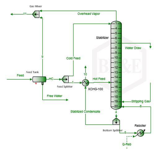
In order to study the effect of CO2, stripping gas rate and TEG mass circulation ratio on the TEG vaporization losses, the TEG dehydration process was simulated using ProMax [2] software with its Soave-Redlich-Kwong (SRK) [3] equation of state (EOS). The process flow diagram used for these simulations is the same as in the November 2013 TOTM [4] and is shown in Figure 1.
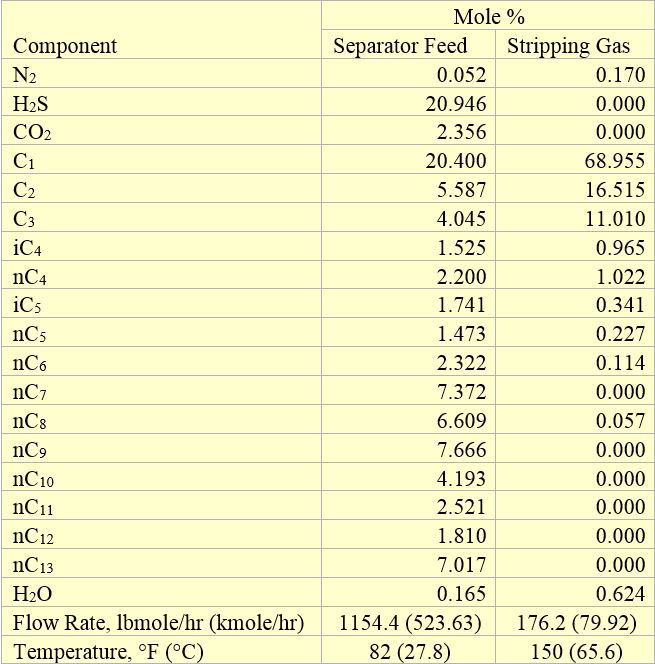
The water-saturated gas with a water content of 915 kg/106 std m3 (57 lbm/MMSCF) enters the bottom of the contactor column at 37.8°C (100°F) and 6897 kPaa (1000 psia) at a rate of 2.835×10⁶ std m3/d (100 MMSCFD). The feed gas studied was either sweet or contained 10 mole % CO2. The contactor column has three theoretical trays. The lean TEG solution enters at the top of the contactor column and flows down in the column. As shown in Figure 1, the water content of the dried gas is 10 mg/std m3 (0.63lbm/MMSCF). The rich TEG solution contains 96.1 mass percent TEG entering the still column at 100°C (212°F) and 515 kPaa (74.7 psia). The reboiler temperature was set at 204.4°C (400°F) and boil-up ratio of 0.1 (molar bases). Two theoretical trays in the regenerator (still) column (NR = 2) and two theoretical trays (NS = 2) in the striping gas section were utilized. The striping gas enters the bottom of the stripping gas section at 204°C (399°F) and 524 kPaa (76 psia). Methane was used for the stripping gas at a rate of 53.6 std m3/h (1893 scf/hr). The regenerated lean solution contains 99.86 mass percent TEG and the ratio of stripping gas to lean TEG liquid volume rates is 20 std m3 of gas/std m3 of lean TEG solution (2.67scf/sgal) or a mass ratio of 28.3. The regenerator (still) top temperature is 91.4°C (196.5°F). If the same stripping gas was sparged directly into the reboiler (NS = 0, no stripping column), with everything else remaining the same, the regenerated solution contains 99.2 mass percent TEG and the regenerator column top temperature remains practically the same and is 91.1°C (196°F). For the above case (NS = 2) the number of theoretical trays in the still column is increased from 2 to 3 (NR = 3); the lean TEG concentration increased slightly from 99.6 to 99.8 mass percent but the regenerator column top temperature remained the same.
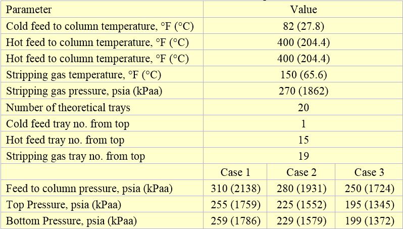
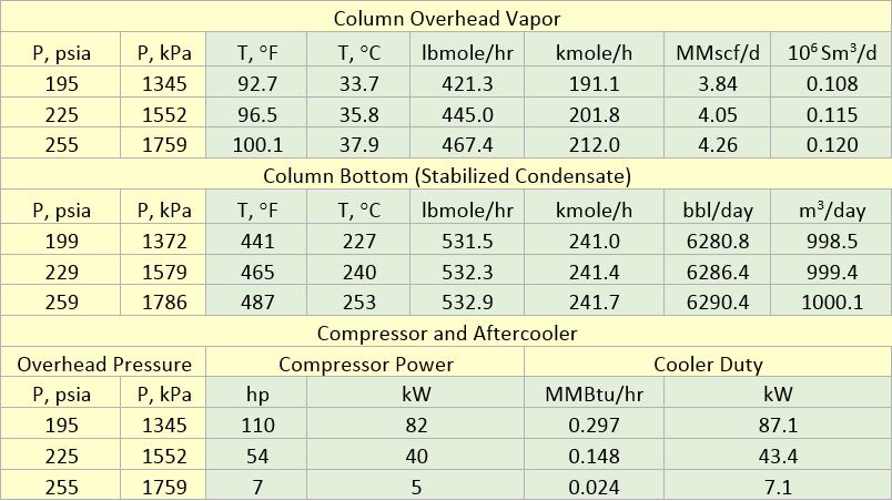
Using a similar set up as is shown in Figure 1, several simulations were performed for a range of stripping gas rates, for NR=2, N S=2 and reboiler pressure of 110.3 kPaa (16 psia) and temperature of 204.4°C (400°F). The results of these simulation runs are presented in Figures 2 and 3.

Figure 1. Sample results using ProMax [2] for TEG dehydration with reboiler P=110.3 kPaa (16 psia) with NR=2 and NS=2 [4]
Figure 2 presents the variation of the TEG vaporization losses from still/regeneartor column top with mass circulation ratio and the stripping gas rate. In addtion to the sweet feed gas (solid lines), Figure 2 also presents results for a feed gas containing 10 mole % CO2 identified by the dashed lines.
Figure 2 indicates that as the stripping gas ratio increases the TEG vaporization losses decrease due to the decrease in temperature at the top of the regenerator column. This figure also indicates that as the TEG mass circulation ratio increases, the TEG vaporization losses increases initially due to lower water content of TEG solution, followed by a decreasing trend with the exception for the case of low stripping gas rate. Figure 2 also indicates that the presence of 10 mole % CO 2 in the feed gas has little effect on the TEG vaporization losses from the regenerator column top. Figure 2 can be used for a quick estimate of the TEG vaporization loss from regenerator top for a given stripping gas rate and TEG circulation mass ratio.

Figure 2. Variation of TEG vaporization loss from regenerator top with circulation mass ratio and stripping gas rate at top P=101.3 kPaa (14.7 psia) and reboiler P=110.3 kPaa (16 psia) at 204.4°C (400°F)
As expected Figure 3 indicates that the TEG vaporization loss from the contactor top increases slightly with the stripping gas rate. In addition, this figure shows that as the TEG mass circulation ratio increases beyond 15 mass of TEG/mass of water removed, the TEG losses remain almost constant. The lower mass circulation ratio corresponds to the lower amount of TEG in contractor and lowers vaporization losses.
Figure 3 also shows that the TEG vaporization loss is higher for the feed gas containing 10 mole % CO2(dashed lines) by a factor of about 18%.
The comparison of Figures 2 and 3 indicates that the TEG vaporization loss from the contactor top is almost 10 times higher than the loss from still/regenerator column top.

Figure 3. Variation of TEG vaporization loss from contactor top with circulation mass ratio and stripping gas rate
CONCLUSIONS
This TOTM studied the effect of CO2 in the feed gas, mass circulation ratio, and stripping gas rate on the TEG vaporization losses from the contactor top and regenerator top. The charts exhibited a quick estimation of the TEG vaporization losses from still/regenerator column top and contactor top at a specified stripping gas rate and TEG mass circulation ratio to achieve the desired level of lean TEG concentration. These are based on the rigorous calculations performed by computer simulations and can be used for facilities type calculations for evaluation and troubleshooting of an operating TEG dehydration unit. In addition, the following observations were made for the cases studied in this TOTM:
>>The TEG vaporization loss from the contactor top is almost 10 times higher than still/regenerator column top (see Figures 2 and 3).
>>Presence of 10 mole % CO2 in the feed gas to contactor column increases the TEG vaporization loss from the top of contactor columns (Figures 3) but has a small effect on TEG vaporization loss from the regenerator column (Figure 2).
>>The results of vaporization loss from the flash tank separator were very small, in the order of 0.0025 lit of TEG/106 Std m3 of gas (0.00002 gal of TEG/MMscf of gas).
>>Though not studied in this TOTM, mechanical losses such as entrainment from contactor top and regenerator top, as well as leaks from pump seals are usually much higher than the vaporization losses presented here.
To learn more about similar cases and how to minimize operational problems, we suggest attending our G4 (Gas Conditioning and Processing), G5 (Practical Computer Simulation Applications in Gas Processing), and G6 (Gas Treating and Sulfur Recovery) courses.
PetroSkills offers consulting expertise on this subject and many others. For more information about these services, visit our website at http://petroskills.com/consulting, or email us at consulting@PetroSkills.com.
By: Dr. Mahmood Moshfeghian
References
Moshfeghian, M., http://www.jmcampbell.com/tip-of-the-month/2013/12/estimating-teg-vaporization-losses-in-teg-dehydration-unit/, Tip of the Month, December 2013.
ProMax 4.0, Bryan Research and Engineering, Inc., Bryan, Texas, 2017.
Soave, G., Chem. Eng. Sci. Vol. 27, No. 6, p. 1197, 1972.
Moshfeghian, M., http://www.jmcampbell.com/tip-of-the-month/2013/11/estimating-still-column-top-temperature-in-teg-dehydration-unit/, Tip of the Month, November 2013.
Moshfeghian, M., http://www.jmcampbell.com/tip-of-the-month/2013/09/high-pressure-regeneration-of-teg-with-stripping-gas/, Tip of the Month, September 2013.


 Figure 9
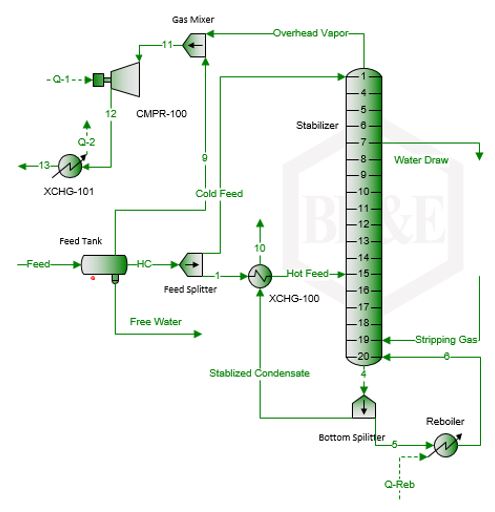

hi