Transportation of CO2 in Dense Phase

 In this tip of the month (TOTM) we will discuss transportation of carbon dioxide (CO₂) in the dense phase. We will illustrate how thermophysical properties change in the dense phase and their impacts on pressure drop calculations. The pressure drop calculations results utilizing the liquid phase and vapor phase equations will be compared. The application of dense phase in the oil and gas industry will be discussed briefly. In a future TOTM, we will discuss the dense phase transportation of natural gas.

When a pure compound, in gaseous or liquid state, is heated and compressed above the critical temperature and pressure, it becomes a dense, highly compressible fluid that demonstrates properties of both liquid and gas. For a pure compound, above critical pressure and critical temperature, the system is oftentimes referred to as a “dense fluid” or “super critical fluid” to distinguish it from normal vapor and liquid (see Figure 1 for carbon dioxide in December 2009 TOTM [1]). Dense phase is a fourth (Solid, Liquid, Gas, Dense) phase that cannot be described by the senses. The word “fluid” refers to anything that will flow and applies equally well to gas and liquid. Pure compounds in the dense phase or supercritical fluid state normally have better dissolving ability than do the same substances in the liquid state. The dense phase has a viscosity similar to that of a gas, but a density closer to that of a liquid. Because of its unique properties, dense phase has become attractive for transportation of CO₂ and natural gas, enhanced oil recovery, food processing and pharmaceutical processing products.

The low viscosity of dense phase, super critical carbon dioxide (compared with familiar liquid solvents), makes it attractive for enhanced oil recovery (EOR) since it can penetrate through porous media (reservoir formation). As carbon dioxide dissolves in oil, it reduces viscosity and oil-water interfacial tension, swells the oil and can provide highly efficient displacement if miscibility is achieved. Additionally, substances disperse throughout the dense phase rapidly, due to high diffusion coefficients. Carbon dioxide is of particular interest in dense-fluid technology because it is inexpensive, non-flammable, non-toxic, and odorless. Pipelines have been built to transport CO₂ and natural gas in the dense phase region due to its higher density, and this also provides the added benefit of no liquids formation in the pipeline.

In the following section we will illustrate the pressure drop calculations for transporting CO₂ in dense phase using liquid phase and vapor phase pressure drop equations.

Case Study:

For the purpose of illustration, we considered a case study for transporting 160 MMSCFD (4.519×10⁶ Sm³/d) CO₂ using a 100 miles (160.9 km) long pipeline with an inside diameter of 15.551 in (395 mm). The corresponding mass flow rate is 214.7 lb_m/sec (97.39 kg/s). The inlet conditions were 2030 psia (14 MPa) and 104˚F (40˚C). The following assumptions were made:

1. Pure CO₂, ignored any impurities such as N₂.
2. Horizontal pipeline, no elevation change.
3. Inside surface relative roughness (roughness factor), ε/D, is 0.00004.
4. Isothermal transportation of CO₂.

Properties: Dense phase behavior is unique and has special features. The thermophysical properties in this phase may vary abnormally. Care should be taken when equations of state are used to predict thermophysical properties in dense phase. Evaluation of equations of state should be performed in advance to assure their accuracy in this region. Many simulators offer the option to use liquid-based algorithms (e.g. COSTALD [2]) for this region. Dense phase is a highly compressible fluid that demonstrates properties of both liquid and gas. The dense phase has a viscosity similar to that of a gas, but a density closer to that of a liquid. This is a favorable condition for transporting CO₂ and natural gas in dense phase as well as carbon dioxide injection into crude oil reservoir for enhanced oil recovery.

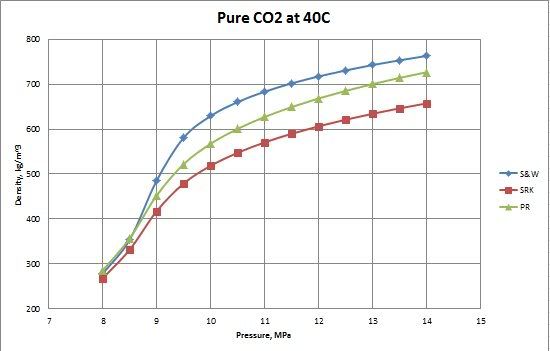
Figures 1 and 2 present variation of density and viscosity of CO₂ with pressure at constant temperature of 104 ˚F (40 ˚C) calculated by the SRK EOS and COSTALD liquid density option in ProMax [3] and the Span and Wagner CO₂  EOS in REFPROP [4] software. Note, ProMax also has the Span and Wagner CO₂  EOS option which produced practically the same results as the REFPPROP.

Figure 1. Density-Pressure diagram for CO₂ at 104˚F (40˚C) by the SRK EOS and COSTALD liquid in ProMax and Span and Wagner CO₂  EOS in REFPROP

Figure 2. Viscosity-Pressure diagram for CO₂ at 104˚F (40˚C) by the SRK EOS and COSTALD liquid in ProMax and Span and Wagner CO₂  EOS in REFPROP

For the sake of easier calculation steps, these diagrams were fitted to the following 3^rd degree polynomials for density and viscosity, respectively:

In these equations, ρ is density (kg/m³), µ is viscosity (cP) and P_avg is the average pipeline segment pressure calculated by:

The fitted coefficients for equations 1 and 2 are presented in Table 1.

Table 1. The fitted coefficients for CO₂ density and viscosity (Equations 1 & 2) at 104˚F (40˚C)

Figures 1 and 2 clearly indicate that there are large differences between predicted properties using two different sources. In the following section, we will illustrate the impact of these differences on pressure drop calculations.

Liquid Phase Pressure Drop Equations: The pressure drop for a liquid phase is calculated as follows.

Where:

Vapor Phase Pressure Drop Equations: In addition to Equations 5 through 8, which are also valid and used for the gas pipeline, the following equations are also used.

Where:

Results and Discussions:

The pressure drop calculations were performed using the liquid phase and vapor phase equations. First, the pipeline cross sectional area was calculated with Equation 8 and the gas density at the standard condition was calculated with equation 10.  In each case the calculation was trial and error and the following step-by-step procedure was followed:

1. The line was divided into n segments (e.g. n = 1, 10, 20, or 100).
2. For segment 1, an outlet pressure was guessed.
3. Segment average pressure was calculated with Equation 3.
4. CO₂ density and viscosity were calculated using Equations 1 and 2, respectively.
5. CO₂ velocity was calculated with Equation 7.
6. Reynolds number was calculated with Equation 6.
7. Friction factor was calculated with Equation 5 (this is also trial and error).
8. Liquid phase pressure drop was calculated with equation 4.
9. Calculate average gas compressibility factor with equation 11.
10. Calculate segment gas outlet pressure by Equation 9 and segment pressure drop with Equation 12.
11. If the calculated outlet pressure is not the same as the guessed outlet pressure in step 2, replace the guessed outlet pressure with the calculated outlet pressure and repeat steps 3 through 10 until the calculated outlet pressure becomes equal to the guessed value.
12. Use the calculated outlet pressure of segment “1” for the inlet of segment “2” and repeat the above steps for each segment till the end of line is reached.

Table 2 summarizes the pressure drop calculation results for four cases in which the pipeline was divided into 1, 10, 20, and 100 segments. Table 2 indicates that for the cases of 10 segments and higher no change in pressure drop is observed.

Table 2. Summary of pressure drop calculation results for different number of segments and different sources of properties.

For all cases tested, both the liquid phase and the vapor phase pressure drop equations gave exactly the same pressure drop. Note that there is at least 100 psi (690 kPa) difference in pressure drops calculation using REFPROP (Span and Wagner CO₂ EOS) or ProMax (SRK EOS and COSTALD liquid density) because the EOS options were different. However, the Span and Wagner CO₂ EOS in both software would result in the same pressure drop. A sample calculation in MathCad format is attached: Dense Phase CO2 Pipeline 1 Segment ProMax.

Table 3 presents the impact of relative roughness on pressure drop. Typical / generally accepted numbers for relative roughness are (and these are regarded as conservative) for steel pipes are:  new or clean service  =  0.00004, mildly corroded  =   0.0002, corroded / dirty service =  0.0004.

Table 3. Impact of relative roughness on pressure drop (Number of segments=10).

Conclusions:

As discussed in December 2009, dense phase behavior is unique and has special features. The thermophysical properties in this phase may vary abnormally. Care should be taken when equations of state are used to predict thermophysical properties in dense phase. Evaluation of equations of state should be performed in advance to assure their accuracy in this region. Many simulators offer the option to use liquid-based algorithms (e.g. COSTALD) for this region. It is very important to use the most appropriate option.

Dense phase is a highly compressible fluid that demonstrates properties of both liquid and gas. The dense phase has a viscosity similar to that of a gas, but a density closer to that of a liquid. This is a favorable condition for transporting CO₂ and natural gas in dense phase. It was also found that either the liquid phase or vapor phase pressure drop equations can be used to calculate CO₂ pressure drop in the dense phase. Both set of equations gave exactly the same pressure drop. Due to high density of CO₂ in the dense phase, pressure drop due to elevation change should not be ignored.

To learn more about similar cases and how to minimize operational problems, we suggest attending our G40 (Process/Facility Fundamentals), G4 (Gas Conditioning and Processing), P81 (CO₂ Surface Facilities), and PF4 (Oil Production and Processing Facilities) courses.

By: Dr. Mahmood Moshfeghian

Reference:

1. Bothamley, M.E. and Moshfeghian, M., “Variation of properties in the dese phase region; Part 1 – Pure compounds,” http://www.jmcampbell.com/tip-of-the-month/2009/12/variation-of-properties-in-the-dense-phase-region-part-1-pure-compounds/, December 2009.
2. Hankinson, R. W., Thomson, G. H., AIChE J., Vol. 25, no. 4, pp. 653-663, 1979.
3. ProMax 3.2, Bryan Research and Engineering, Inc, Bryan, Texas, 2011.
4. NIST Reference Fluid Thermodynamic and Transport Properties Database (REFPROP): Version 9.0, 2011.