Lean Sweet Natural Gas Water Content Correlation

In the October, November, December 2007 and February 2014 Tips of the Month (TOTM), we studied in detail the water phase behaviors of sweet and sour natural gases and acid gas systems. We also evaluated the accuracy of different methods for estimating the water content of sour natural gas and acid gas systems.

The water vapor content of natural gases in equilibrium with water is commonly estimated from Figure 6.1 of Campbell book [1] or Figure 20.4 of Gas Processors and Suppliers Association, including corrections for the molecular weight (relative density) of gas and salinity of water [2].

In this TOTM, we will present two new correlations for estimating the water content of lean and sweet natural gases. The performance of the proposed correlations will be compared with the rigorous simulation and shortcut method software and other correlations.

Low Pressure System

At low pressure conditions, less than 700 kPa (100 psia), the mole fraction of water in the gas phase can be estimated by dividing water vapor pressure, P^V, at the specified temperature, T, by the system pressure, P. The vapor pressure of pure water, from 0 to 360, (32 to 680) can be calculated by the following relation [3].

Where:

The critical temperature, T_C = 647.096 K and critical pressure, P_C = 22.064 MPa, T in K, and P^V in MPa, and

a₁ = −7.85951783,     a₂ = 1.84408259,     a₃ = −11.7866497,      a₄ = 22.6807411,

a₅ = −15.9618719,     a₆ = 1.80122502

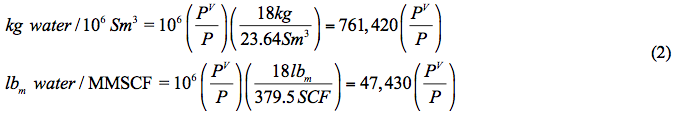
Knowing  one kmole of water = 18 kg (lbmole=18 lb_m) and one kmole of gases occupy 23.64 Sm³ at standard condition of 15  and 101.3 kPa (one lbmole of gases occupy 379.5 SCF at standard condition of 60 and 14.7 psia), the water content is calculated by

Moderate to High Pressure System

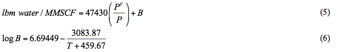
For pressures higher than 700 kPa (100 psia), we propose a correlation similar to equation 6-276 in Chapter 6 of Standard Petroleum Handbook [4] as follows:

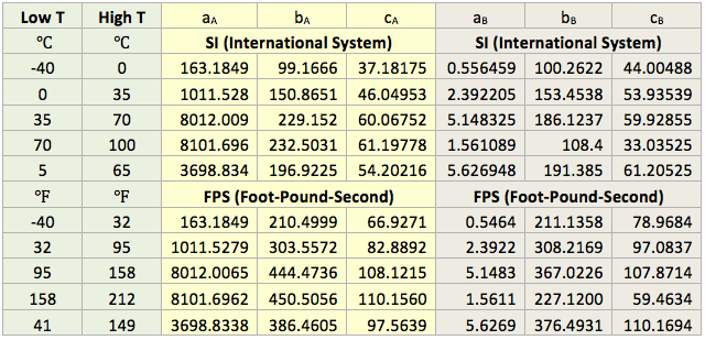
Reference [4] presents the tabular values of A and B as a function of temperature. In this work, the temperature dependency of A and B in equation 3 is presented in the form of Gaussian Model.

Where:

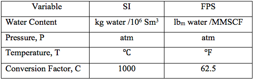
A temperature range of -40 to 100 (-40 to 212) and pressure range of 6.8 to 680 atm have been considered. For the purpose of higher accuracy, the parameters in equations 4G are regressed and presented in Table 1 for 5 different temperature intervals, for SI (System International) and FPS (Foot-pound-Second) system of units. The temperature range in the 5^th row in each system of units is used more frequently. The proposed correlations are suitable for spreadsheet calculations.

            Table 1. The parameters for equation 4G (Gaussian Model).

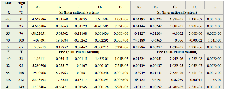
Alternatively, the temperature dependency of parameters A and B in equation 3 can also be presented in the form of Polynomial Model.

Similarly, the correlation parameters of equations 4P are presented in Table 2.

The performance of the proposed correlation was evaluated against the water content of a lean sweet natural gas with a relative density (specific gravity) of 0.6 calculated by SRK equation of state of ProMax software [5]. The water saturator tool of ProMax was utilized. Figure 1A (SI) and Figure 1B (FPS) present the comparison between the proposed correlation (Eqs. 3 and 4G) results (solid curves) and the corresponding results from ProMax designated by geometric symbols.  Figure 1 indicates there is relatively good agreement between the proposed correlation and ProMax. Large deviations are observed for temperatures below -20 (-4). Almost in all conditions, except at very high temperature the proposed correlation is more conservative (over predicting) than the ProMax.

Table 2. The parameters for equation 4P (Polynomial Model).

Evaluation of the Proposed Correlation

The performance of the proposed correlation was also evaluated against the water content of a lean sweet natural gas predicted by GCAP  software [6].  The water content of GCAP is based on Figure 6.1 of Campbell book [1]. Figure 2A (SI) and Figure 2B (FPS) present the comparison between the proposed correlation (Eqs. 3 and 4G) results (solid curves) and the corresponding results from GCAP designated by geometric symbols.  Figure 2 indicates there is better agreement between the proposed correlation and GCAP compared to ProMax. Large deviations are observed for temperatures below -20 (-4). Almost in all conditions, except at very high temperature, the proposed correlation is slightly more conservative (over predicting) than the GCAP.

Figures 1 and 2 indicate that in the temperature range of 0 to 70 (32 to 158 ) excellent agreement is observed between results of equation 3 and both software. Figure 2 also indicates that the GCAP results for 170 atm at very low temperature is inconsistent with other pressure results of GCAP.

When equation 4P and the parameters presented in Table 2 were used instead of equation 4G, similar quality of results was obtained.

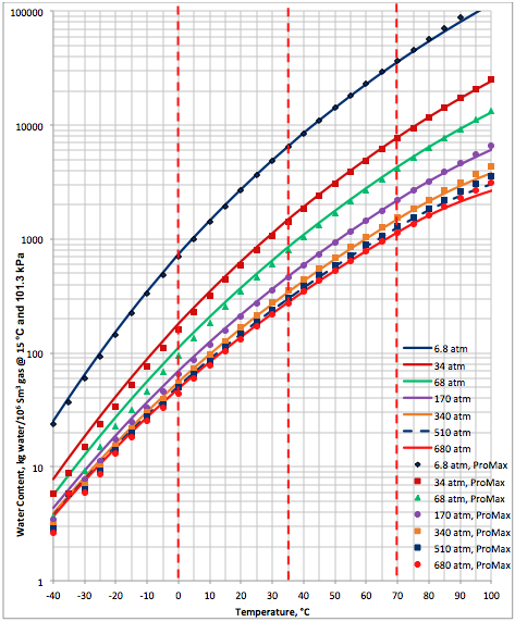
Figure 1A (SI). Comparison of results between the proposed correlation (Eq 3) and ProMax

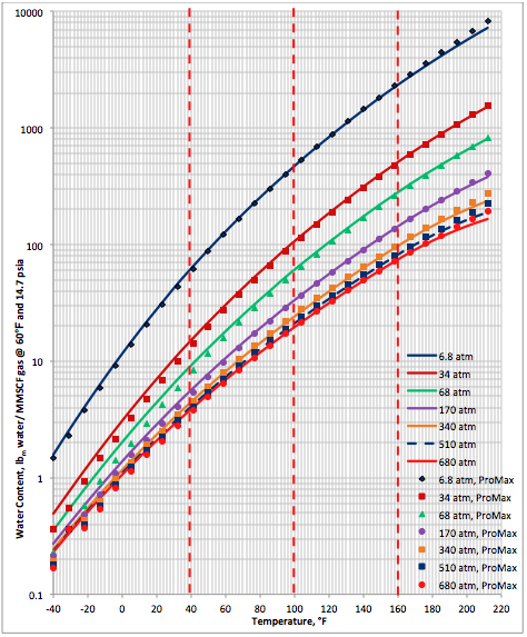
Figure 1B (FPS). Comparison of results between the proposed correlation (Eq 3) and ProMax

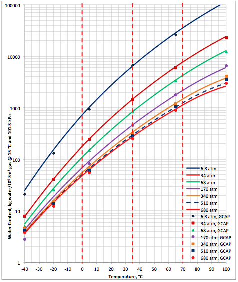
Figure 2A (SI). Comparison of results between the proposed correlation (Eq 3) and GCAP

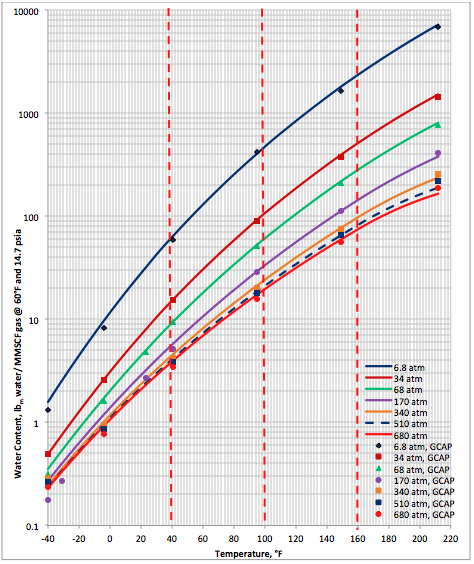
Figure 2B (FPS). Comparison of results between the proposed correlation (Eq 3) and GCAP

Bukacek Correlation

Bukacek [7] suggested a relatively simple correlation for the water content of lean sweet gas as follows:

where T is in °F.

This correlation is reported to be accurate for temperatures between  15.5 and 238°C (60 and 460°F) and for pressure from 0.105 to 69.97 MPa (15 to 10,000 psia). The pair of equations in this correlation is simple in appearance. The added complexity that is missing is that it requires an accurate estimate of the vapor pressure of pure water. In this study, we have used equation 1 for water vapor pressure.

The performance of the proposed correlation was also evaluated against the Bukacek’s Correlation coupled with equation 1 for water vapor pressure. Figure 3A (SI) and Figure 3B (FPS) present the comparison between the proposed correlation (Eqs. 3 and 4G) results (solid curves) and the corresponding results from Bukacek’s correlation designated by geometric symbols.  Figure 3 indicates there is an excellent agreement between the proposed correlation and Bukacek’s correlation.

Conclusions

The following conclusions can be made regarding the proposed correlation:

1. A relatively simple correlation for predicting the water content of lean sweet natural gas is presented that can be used for spreadsheet calculation.
2. Based on Figures 1 and 2, the agreement between the predicted water content by the proposed correlation (Eqs. 3 and 4G or Eqs. 3 and 4P) and those predicted by ProMax and GCAP software is relatively good. The agreement deteriorates at temperatures below -20 (-4).
3. In general, the estimated water content by the proposed correlation is conservative compared to ProMax and GCAP.
4. A better agreement between the proposed correlation and GCAP compared to ProMax is observed.
5. Excellent agreement is observed between the proposed and the Bukacek’s correlations.
6. The GCAP results for pressure of 170 atm at low temperatures are inconsistent with respect to GCAP results at other pressure.
7. The proposed correlation is easy and suitable for hand or spreadsheet calculations.

To learn more about similar cases and how to minimize operational problems, we suggest attending our G6 (Gas Treating and Sulfur Recovery), G4 (Gas Conditioning and Processing), PF81 (CO₂ Surface Facilities), PF4 (Oil Production and Processing Facilities), and PL4 (Fundamentals of Onshore and Offshore Pipeline Systems) courses.

John M. Campbell Consulting (JMCC) offers consulting expertise on this subject and many others. For more information about the services JMCC provides, visit our website at www.jmcampbellconsulting.com, or email us at consulting@jmcampbell.com.

By: Dr. Mahmood Moshfeghian

Reference:

1. Campbell, J.M., Gas Conditioning and Processing, Volume 1: The Basic Principles, 9^th Edition, 2^nd  Printing, Editors Hubbard, R. and Snow–McGregor, K., Campbell Petroleum Series, Norman, Oklahoma, 2014.
2. GPSA Engineering Data Book, Section 20, Volume 2, 13^th Edition, Gas Processors and Suppliers Association, Tulsa, Oklahoma, 2012.
3. Wagner, W.  and Pruss, A.,  J. Phys. Chem. Reference Data, 22, 783–787, 1993.
4. Standard Handbook of Petroleum, Natural Gas Engineering volume 2, Lyons, W. C., Editor, Gulf Professional Publishing, Houston, Texas, 1996
5. ProMax 3.2, Bryan Research and Engineering, Inc., Bryan, Texas, 2014.
6. GCAP 9.1, Gas Conditioning  and Processing, PetroSkills/Campbell, Norman, Oklahoma, 2014
7. Bukacek, R.F., “Equilibrium Moisture Content of Natural Gases” Research Bulletin IGT, Chicago, vol 8, 198-200,  1959.

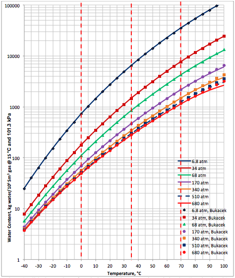
Figure 3A (SI). Comparison of results between the proposed correlation (Eq 3) and Bukacek’s Correlation

Figure 3A (FPS). Comparison of results between the proposed correlation (Eq 3) and Bukacek’s Correlation