Accurate measurement and prediction of crude oil and natural gas liquid (NGL) products vapor pressure are important for safe storage and transportation, custody transfer, minimizing vaporization losses and environmental protection. Vapor pressure specifications are typically stated in Reid Vapor Pressure (RVP) or/and True Vapor Pressure (TVP). In addition to the standard procedures for their measurements, there are rigorous and shortcut methods for their estimation and conversion.
There are figures and monographs for conversion of RVP to TVP for NGLs (Natural Gas Liquids) and crude oil at a specified temperature. This tip will present simple correlations for conversion from RVP to TVP and vice versa at a specified temperature. The correlations are easy to use for hand or spreadsheet calculations. Figures generated using these correlations will be presented, too.
Chapter 5 of reference [1] presents an excellent overview of TVP and RVP including their definitions, standard procedures for their measurements and diagrams for their conversion. The proceeding two paragraphs are extracted with minor revisions from reference [1].
TVP is the actual vapor pressure of a liquid product at a specified temperature and is measured with a sample cylinder. TVP specifications must always be referenced to a temperature, which frequently falls between 30-50°C (86-122°F). TVP is difficult to measure and depends on the ratio of the vapor to liquid, V/L, in the measurement device. If V/L = 0, the vapor pressure is essentially equivalent to the bubble point of the mixture which is the highest vapor pressure value for the liquid. As V/L increases, i.e., a small amount of vapor exists at the point of measurement, the measured vapor pressure will decrease. The relationship between the measured TVP and V/L depends on the composition of the mixture. For “near pure” component mixtures, V/L has little effect on the measured vapor pressure. For mixtures with a large composition range, such as crude oil or condensate, the effect of V/L on the measured vapor pressure can be significant (See ASTM D 6377 – 10 for detail). Reference [1] lists the Standards used for TVP measurements.
Because of the difficulty in accurately measuring TVP, an alternative method of measuring vapor pressure is frequently used. This is the RVP. The RVP is a standard test set out in ISO 3007:1999, Petroleum products and crude petroleum – Determination of vapour pressure – Reid method. Another standard that applies to RVP is: ASTM D323 – 08, Standard Test Method for Vapor Pressure of Petroleum Products (Reid Method). The RVP test is applicable for crude oils, condensates, and petroleum products such as gasoline (petrol) mixtures. A liquid sample is collected in the lower 20% chamber (see Fig 5.12 of reference [1]). The 80% chamber, which is filled with air (may also contain a small amount of water vapor) at atmospheric pressure. Both chambers are cooled to 0°C (32°F). The 80% air chamber (at atmospheric pressure) is then connected to the 20% liquid chamber. The connecting valve is opened and the cylinder is heated in a water bath to 37.8°C (100°F). The pressure indicated on the gauge is the RVP.
Reference [1] provides Figure 5.14 for conversion RVP to TVP for motor gasoline (petrol) and natural gasoline (C5+ NGLs) at various temperatures. Figure 5.15 of reference [1] is a nomograph that shows the approximate relationship between RVP and TVP for crude oil. It is commonly used for converting RVP to TVP at custody transfer points where the vapor pressure specification for the oil is a TVP, but the actual vapor pressure measurement is an RVP.
Vazquez-Esparragoza et al. [2] present an algorithm to calculate RVP without performing the actual test. The algorithm, based on an air-and-water free model, uses the Gas Processors Association Soave-Redlich-Kwong [3] equation of state and assumes liquid and gas volumes are additive. This algorithm can be used to predict RVP of any hydrocarbon mixture of known composition. Since the calculations are iterative, it should be incorporated into a general purpose process simulator. Vazquez-Esparragoza et al. [2] reported good agreement between predicted and experimental values.
Riazi et al. [4] presented a new correlation for predicting the RVP of gasoline and naphtha based on a TVP correlation. The input parameters for this correlation are the mid-boiling point, specific gravity, critical temperature, and critical pressure, where the critical properties may be estimated from the boiling point and specific gravity using available methods. They evaluated their proposed correlation with data collected on 50 gasoline samples from crude oils from around the world with API gravity ranges from 41 to 87, average boiling point ranges from 43 to 221 °C (110 to 430 °F) and RVP of 0.7 to 115 kPa (0.1–17 psi). The average error from their proposed correlation is about 6 kPa (0.88 psi) [4].
Development of Model for Motor Gasoline and Natural Gasoline
To develop the desired correlations for conversion of motor gasoline and natural gasoline RVP to TVP and vice versa, this tip generated 127 data points from Figure 5.14 of reference [1]. These data covered the full ranges of temperature, RVP and TVP of Figure 5.14.
RVP to TVP: This tip used these data to determine the parameters to the Equations 1 through 3. The API 2517 originally reported the same forms of equations for crude oil.
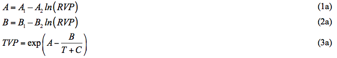
TVP to RVP: Similarly this tip proposes the following equations for conversion from TVP to RVP.
where:
T = Temperature, °C (°F)
RVP = Reid Vapor Pressure, kPa (psi)
TVP = True Vapor Pressure, kPaa (psia)
Note that the values of A1, A2, B1, and B2 are different in the above two sets of equations. The value of “C” is a function of the chosen units (SI versus FPS) and is consistent.
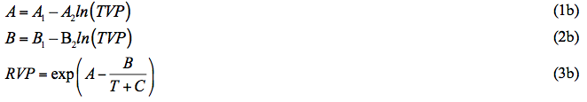
Table 1 presents the optimized values of A1, A2, B1, B2, and C for three sets of data in FPS (Foot-Pound-Second) and SI (System International). The data set labeled “All” included 127 data points covering all of the data of combined motor gasoline and natural gasoline. The data set “Motor Gasoline’ and “Natural Gasoline’ cover 76 and 51 data points for motor gasoline and natural gasoline, respectively. Table 1 also presents the Average Absolute Percent Deviation (AAPD), the Maximum Absolute Percent Deviation (MAPD), Average Absolute Deviation (AAD), and the number of data points (NP) for each data set. The error analysis of Table 1 indicates that the accuracy of the proposed correlations is good. Their accuracy is as good as the quality of tabular data generated from Figure 5.14.
Table 1. The optimized parameters for motor gasoline and natural gasoline
1AAPD = Average Absolute Percent Deviation
2MAPD = Maximum Absolute Percent Deviation
3AAD = Average Absolute Deviation
4NP = Number of data Points (NP)
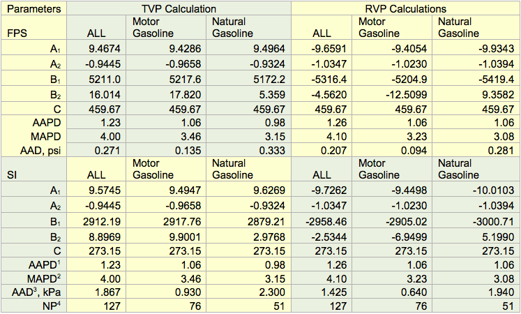
Figures 1a (SI) and 1b (FPS) present the tabular data (generated from Figure 5.14 of reference [1]) in the form of “legends”. This figure also presents the predicted TVP by the proposed correlations (Equations 1 through 3 and the corresponding parameters listed in Table 1) as a function of temperature and RVP in the form of “continuous lines” and “broken lines” for motor gasoline and natural gasoline, respectively.
Figure 1a. TVP as a function of RVP and temperature for motor gasoline and natural gasoline (typical C5+ NGLs)
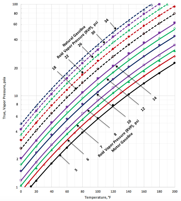
Figure 1b. TVP as a function of RVP and temperature for motor gasoline and natural gasoline (typical C5+ NGLs)
Development of Model for Crude Oil
To develop the desired correlations for conversion of crude oil RVP to TVP and vice versa, this tip generated 196 data points from Figure 5.15 of reference [1] using the correlations reported in API 2517. The API 2517 equations are the same as shown in Equations 1 through 3. These data covered the full ranges of temperature, RVP and TVP of Figure 5.15.
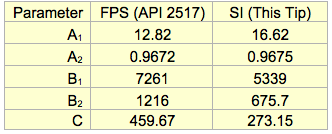
RVP to TVP: Table 2 presents the API 2517 FPS parameters of A1, A2, B1, B2, and C for Equations 1a, 2a, and 3a (T, °F, RVP, psi and TVP, psia). This tip determined the SI (T, °C, RVP, kPa and TVP, kPaa) corresponding parameters. Table 2 also presents the SI parameters.
Table 2. API 2517 parameters for crude oil TVP calculations
(For use with Equations 1a, 2a and 3a)
Figures 2a (SI) and 2b (FPS) present the predicted TVP by Equations 1a, 2a and 3a and the corresponding parameters listed in Table 2 as a function of temperature and RVP for crude oil.
TVP to RVP: To cover the full ranges of Figure 5.15 of reference [1], this tip proposes the following equations for conversion of TVP to RVP.
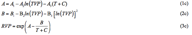
where:
T = Temperature, °C (°F)
RVP = Reid Vapor Pressure, kPa (psi)
TVP = True Vapor Pressure, kPaa (psia)
Table 3 presents the optimized values of A1, A2, A3, B1, B2, B3, and C for RVP calculation in FPS and SI for the proposed Equations 1c through 3c. Table 3 also presents the Average Absolute Percent Deviation (AAPD), the Maximum Absolute Percent Deviation (MAPD), Average Absolute Deviation (AAD), and the Number of data Points (NP). The error analysis of Table 3 indicates that the accuracy of the proposed correlations is good and can be used for the estimation purposes.
Table 3. The optimized parameters for crude oil TVP conversion to RVP
(For use with Equations 1c, 2c & 3c)
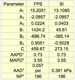
1AAPD = Average Absolute Percent Deviation
2MAPD = Maximum Absolute Percent Deviation
3AAD = Average Absolute Deviation
4NP = Number of data Points (NP)
Conclusions:
For converting RVP to TVP of motor gasoline and natural gasoline, this tip presented simple correlations similar to the ones reported in API 2517 for crude oil RVP to TVP. This tip determined the correlation parameters by regressing the data generated from available diagrams. These correlations were also extended for easy conversion from TVP to RVP. Tables 1, 2, and 3 present the correlation parameters in SI and FPS system of units. Tables 1 and 3 presents the accuracy of the proposed correlations against the data generated from diagrams. Tables 1 and 3 indicate that the accuracy of these correlations is as good as the quality of the data in the original diagram and can be used for easy conversion of RVP to TVP or vice versa. These correlations are easy to use for hand or spreadsheet calculations and should be used for estimation purposes. For accurate measurements, correction procedures outlined in ASTM D 6377–10 and other guidelines should be consulted. Several organizations are currently working to improve the accuracy of TVP estimation from RVP and/or VPCR(x) (ASTM D6377) measurement techniques. In all cases, Federal and State Laws and Regulations should be followed for safety and environmental protection.
To learn more about similar cases and how to minimize operational problems, we suggest attending our G4 (Gas Conditioning and Processing), G5 (Advanced Applications in Gas Processing), and PF4 (Oil Production and Processing Facilities), courses.
PetroSkills offers consulting expertise on this subject and many others. For more information about these services, visit our website at http://petroskills.com/consulting, or email us at consulting@PetroSkills.com.
By: Dr. Mahmood Moshfeghian
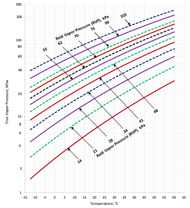
Figure 2a. TVP as a function of RVP and temperature for crude oil
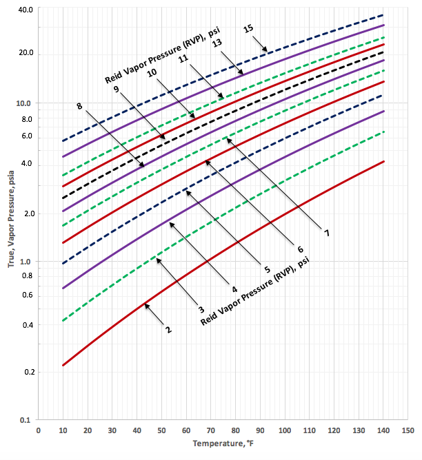
Figure 2b. TVP as a function of RVP and temperature for crude oil
References:
- Campbell, J.M., Gas Conditioning and Processing, Volume 1: The Basic Principles, 9th Edition, 2nd Printing, Editors Hubbard, R. and Snow–McGregor, K., Campbell Petroleum Series, Norman, Oklahoma, 2014.
- Vazquez-Esparragoza, J.J., et al, “How to Estimate Reid Vapor Pressure (RVP) of Blends”, Bryan Research and Engineering, Inc, Bryan, Texas, 2015.
- Soave, Chem. Eng. Sci. 27, 1197-1203, 1972.
- Riazi, M.R., Albahri, T.A. and Alqattan, A.H., “Prediction of Reid Vapor Pressure of Petroleum Fuels”, Petroleum Science and Technology, 23: 75–86, 2005.

![Figure 1. A simplified process flow diagram for a two-tower adsorption dehydration system [1].](http://www.jmcampbell.com/tip-of-the-month/wp-content/uploads/2015/10/fig1.png)
![Figure 2. A simplified process flow diagram for a three-tower adsorption dehydration system [1].](http://www.jmcampbell.com/tip-of-the-month/wp-content/uploads/2015/10/fig2.png)
![Figure 1. A simplified process flow diagram for a 3-tower adsorption dehydration system [1].](http://www.jmcampbell.com/tip-of-the-month/wp-content/uploads/2015/09/fig1.png)
![Figure 1. Schematic of the forces acting on a liquid droplet in the gas phase [5]](http://www.jmcampbell.com/tip-of-the-month/wp-content/uploads/2015/08/fig1.png)
![Figure 2. KS as a function of pressure and liquid droplet size for vertical separators with no mist extractor devices [5]](http://www.jmcampbell.com/tip-of-the-month/wp-content/uploads/2015/08/fig2.png)
![Figure 3. Schematic of a horizontal gas-liquid separator [5]](http://www.jmcampbell.com/tip-of-the-month/wp-content/uploads/2015/08/fig3.png)
![Figure 4. Typical mist extractor in a vertical separator [5]](http://www.jmcampbell.com/tip-of-the-month/wp-content/uploads/2015/08/fig4.png)
![Figure 1. Schematic of the forces acting on a liquid droplet in the gas phase [5]](http://www.jmcampbell.com/tip-of-the-month/wp-content/uploads/2015/08/appfig1.png)


![Figure 1. Typical process flow diagram for a 2-tower adsorption dehydration system [1]](http://www.jmcampbell.com/tip-of-the-month/wp-content/uploads/2015/04/Fig1.png)
![Figure 2. Typical process flow diagram for a 3-tower adsorption dehydration system [1]](http://www.jmcampbell.com/tip-of-the-month/wp-content/uploads/2015/04/Fig2.png)
![Figure 3. A generic molecular sieve decline curves [1]](http://www.jmcampbell.com/tip-of-the-month/wp-content/uploads/2015/04/Fig3.png)
![Figure 4. Design condition life factor [1]](http://www.jmcampbell.com/tip-of-the-month/wp-content/uploads/2015/04/fig41.png)
![Figure 5. Performance test run (PTR) life factor [1]](http://www.jmcampbell.com/tip-of-the-month/wp-content/uploads/2015/04/fig5.png)
![Figure 6. Projected life factor (red triangle) running at design conditions [1]](http://www.jmcampbell.com/tip-of-the-month/wp-content/uploads/2015/04/fig6.png)
![Figure 7. Projected life factor running at design conditions [1]](http://www.jmcampbell.com/tip-of-the-month/wp-content/uploads/2015/04/fig71.png)
![Figure 8. Projected life factor (red triangle) if standby time is used [1]](http://www.jmcampbell.com/tip-of-the-month/wp-content/uploads/2015/04/fig81.png)

Good site you have got here.. It’s difficult to find high-quality writing like yours nowadays. I truly appreciate individuals like you! Take care!!|
Dear Prof.
This is a nice piece of work, and is useful for students of chemical engineering, as well as process engineers
Please include my email in the new tip of the month topics
Great post! Have nice day ! 🙂 jhqqd
Hello
Why the RVP test in temperature 37.8 C ?
Normally RVP is measured at 100 F which i the same as 37.8 C.
[…] Correlations for Conversion between True and Reid Vapor. – Accurate measurement and prediction of crude oil and natural gas liquid (NGL) products vapor pressure are important for safe storage and transportation, custody. […]
Thank you a lot for giving your thoughts. Other then that, great post! Might there be any scientific papers on this subject or any closely related topics? Keep up the cool quality writing, it is rare to see a nice post like this one these days. Wow, that sure is a smart way of thinking about it.