For dehydration of natural gas by triethylene glycol (TEG) process to a lower water content/water dew point temperature a higher lean TEG concentration is required. To achieve a higher lean TEG concentration at a specified reboiler temperature and pressure, commonly a stripping gas is used. Stripping is defined as a physical separation process by which one or more components are removed from a liquid stream by a vapor stream. Stripping gas lowers the water partial pressure causing more water to vaporize from TEG solution. Normally, stripping is performed at the practical/possible highest temperature and lowest pressure. This allows for minimum stripping gas flow rate. Any inert gas or a portion of the gas being dehydrated is suitable.

In this Tip Of The Month (TOTM), the impact of stripping gas on the water partial pressure and lean TEG solution boiling temperature or lean TEG concentration is studied. Two case studies are considered. In case one, at a specified reboiler temperature and pressure, the impact of stripping gas on lowering the water partial pressure and consequently increasing the TEG concentration in the lean TEG solution is demonstrated. Similarly in case two, for a specified 99 and 99.4 mass percent TEG in the liquid phase and atmospheric pressure, the impact of stripping gas on lowering the water partial pressure and consequently lowering the liquid boiling point (bubble point) temperature is demonstrated.

Glycol dehydration is the most common dehydration process used to meet pipeline sales specifications and field requirements (gas lift, fuel, etc.). TEG is the most common glycol used in these absorption systems. At atmospheric pressure and a maximum reboiler temperature of 204 °C [400 °F] the highest glycol concentration of lean TEG that can be achieved is roughly 99 mass percent. This represents the maximum lean TEG concentration that can be produced in a reboiler operating at 1 atm. If the lean TEG concentration required at the absorber to meet the water dew point specification is higher than 99 mass percent, then some method of further increasing the glycol concentration at the regenerator must be incorporated in the unit. Virtually all of these methods involve lowering the partial pressure of water in the glycol solution either by pulling a vacuum on the regenerator or by introducing stripping gas into the regenerator [1].

In the June and July 2013 Tip Of The Months (TOTM) [2, 3], the effect of stripping gas rate on the regenerated lean TEG concentration for several operation conditions was studied. A series of charts and their corresponding correlations for quick determination of the required stripping gas rate to achieve a desired level of lean TEG concentration were presented. The charts were based on the rigorous calculations performed by computer simulations with correlations developed by regressing the same data to a proposed model. These can be used for facilities type calculations for evaluation and trouble shooting of an operating TEG dehydration unit. For further detail refer to the June and July 2013 TOTM [2, 3].

Vapor-Liquid Equilibrium:

For the sake of simplicity, pure methane is used as the stripping gas; however, the following discussion is valid for any gas mixture.

The governing equations for vapor-liquid equilibrium of TEG, water, and methane are derived and presented in Appendix A at the end of this TOTM. Even though the system of water, TEG and methane is non-ideal, to show the principle of gas stripping, assume the vapor phase is an ideal gas and the liquid phase is an ideal solution. Under these conditions Raoult’s Law for water (See Eq A5 in Appendix A) is.

According to Raoult’s Law, at a fixed pressure and temperature (i.e. the reboiler condition), the mole fraction of water in the liquid phase (x_water) decreases as water partial pressure decreases. Note that at a fixed temperature, water vapor pressure is constant (see Figure 1). In addition, system pressure (P) is the sum of partial pressure of all components. Assuming an ideal mixture, mathematically P is approximated by:

Figure 1 presents the vapor pressure of water [4] and TEG [5] for an operating range of reboiler temperature. As can be seen in Figure 1, the vapor pressure (volatility) of water is much higher than that of TEG. In general the vapor pressure of water is approximately 100 to 1000 times greater than that of TEG. This shows why water is vaporized much more than TEG from a TEG solution by heating.

Since TEG volatility is much lower than that of water and methane, its mole fraction in the vapor phase will be much smaller and for simplicity its partial pressure can be ignored. Therefore equation 2 reduces to:

At a fixed system pressure (reboiler condition), equation 3 clearly shows that as the methane partial pressure increases, water partial pressure has to decrease and consequently, based on Raoult’s Law, equation 1, the mole fraction of water in the liquid phase decreases. In other words, increasing the stripping gas rate results in lower water mole fraction in TEG and higher TEG mole (mass) fraction is achieved.

Fig 1A (SI). Comparison of water [4] and TEG [5] vapor pressure

Fig 1B (FPS). Comparison of water [4] and TEG [5] vapor pressure

The effect of stripping gas can be summarized as follows:

• Higher stripping gas (methane) rate increases methane mole fraction in the vapor phase
• Higher methane mole fraction in the vapor phase increases partial pressure of methane
• Higher partial pressure of methane lowers partial pressure of water (P is fixed, Eq 3)
• Lower partial pressure of water lowers mole fraction of water (Raoult’s Law, Eq 1) in the liquid phase (Raoult’s Law, Eq 1) which, in turn, increases the TEG concentration

In order to demonstrate quantitatively the impact of stripping gas on water partial pressure and lean TEG concentration or boiling temperature and to support the above reasoning, two case studies were investigated. For both cases, ProMax [6] with the SRK (Soave-Redlich-Kwong) [7] equation of state option was used to perform the calculations. In addition, all of the results presented are are for a single equilibrium (theoretical) stage.

Case Study 1:

In this case, the impact of stripping gas on regeneration of lean TEG concentration at reboiler conditions of 101.3 kPa and 199°C (14.7 psia & 390°F) is studied.

Figures 2 A & B present the variation of partial pressures of TEG, water and methane as a function of stripping gas (methane) rate and concentration, respectively. The total pressure is constant and plotted in this figure as well. These figures clearly show that as stripping gas (methane) rate or concentration increases, the methane partial pressure increases and the water partial pressure decreases, approximately in the same amount. Note the TEG partial pressure is relatively constant and very low compared to methane and water. It makes up less than 7 percent of the total pressure.

Figures 3 A & B present the impact of stripping gas rate and concentration in the vapor and liquid phases on lean TEG concentrations. As can be seen in these figures, as the stripping gas rate (or concentration) increases, the lean TEG concentration increases. It should be emphasized that these results are for a single equilibrium stage. As shown in the previous TOTM, increasing the number of stripping stages changes this relationship significantly.

Figures 2 and 3 indicate that variation of methane and water partial pressures or lean TEG concentration with stripping gas (methane) rate is non-linear whereas their variation with stripping gas concentration is linear.

Fig 2A. Impact of stripping gas rate on partial pressure of methane, water and TEG at 101.3 kPa & 199°C (14.7 psia & 390°F)

Fig 2B. Impact of stripping gas concentration on partial pressure of methane, water and TEG at 101.3 kPa & 199°C (14.7 psia & 390°F)

Fig 3A. Impact of stripping gas rate on lean TEG concentration at 101.3 kPa & 199°C (14.7 psia & 390°F)

Fig 3B. Impact of stripping gas concentration on lean TEG concentration at 101.3 kPa & 199°C (14.7 psia & 390°F)

Case Study 2:

This is an academic case and is presented to reemphasize the impact of stripping gas. In this case, the impact of stripping gas concentration on the lean TEG solution boiling (bubble point) temperature for relatively fixed lean TEG concentration of TEG and water at 101.3 kPa (14.7 psia) is studied.

Figure 4 indicates that as the stripping gas (methane) concentration increases, the lean TEG solution boiling (bubble point) temperature drops.

Figure 5 presents a variation of partial pressures of TEG, water and methane as a function of the stripping gas (methane) concentration. The total pressure is constant and plotted in this figure, too. As in case 1, this figure also clearly indicates that as the stripping gas (methane) concentration increases, while methane partial pressure increases water partial pressure decreases, approximately in the same amount. Note that TEG partial pressure decreases due to the lowering of boiling temperature and its value is much lower compared to those of methane and water. Again, it makes up less than 7 percent of total pressure.

Variation of component K-values as a function of TEG solution boiling (bubble point) temperature is presented in Figure 6. This figure indicates that the relative volatility of water with respect to TEG (K_water/K_TEG) is in the order of 100 and that of methane with respect to TEG (K_methane/K_TEG) is in the order of more than 10,000.

Fig 4. Impact of stripping gas concentration on the lean TEG solution boiling (bubble point) temperature at 101.3 kPa (14.7 psia).

Fig 5. Impact of stripping gas concentration on the component partial pressures at 101.3 kPa (14.7 psia) for 99 mass % TEG and 1 mass % water.

Fig 6. Variation of K-values with the lean TEG solution boiling (bubble point) temperature at 101.3 kPa (14.7 psia) for 99 mass % TEG and 1 mass % water.

Example 1:

Determine the reboiler temperature to regenerate a lean TEG concentration of 99.4 mass % at 101.3 kPa (14.7 psia). If the required reboiler temperature is above the maximum allowable of 204°C (400°F), determine the required partial pressure of a stripping gas (methane) to keep the reboiler temperature at 199°C (390°F).

Solution:

Figure 4 indicates that for a lean TEG concentration of 99.4 mass %, the required reboiler temperature without any stripping gas is 220.5°C (428.8°F). Obiviously, the is above the maximum allowable operating reboiler temperature. From the same figure, for a reboiler temperature of 199°C (390°F), the required mole % of striping gas in the vapor phase is 35.6. Therefore, the required partial of stripping gas is:

Example 2:

It is desired to regenerate a lean TEG solution to a concentration of 99.4 mass % at 101.3 kPa and 199°C (14.7 psia & 390°F). How much stripping gas is required in a regenerator with 1 theoretical tray?

Soultion:

Figure 3A indicates that for a lean TEG concentration of 99.4 mass%, the required striping gas rate is 10.9 Std m³/m³ of TEG (1.44 SCF/gal TEG). The coressponding water and methane partial pressures from Figure 2A are 57.8 and 36.5 kPa ( 8.4 and 5.3 psia), respectively. Note that without any stripping gas, the maximum achievable lean TEG concentration is 99 mass % and the coressponding water and methane partial pressures are 94.6 and 0 kPa (13.7 and 0 psia), respectively. The stripping gas reduced the water partial presuure by 38.9 %.

Conclusions:

 To achieve a higher lean TEG concentration at a specified reboiler temperature, i.e. below maximum of 204°C (400°F), and pressure, a stripping gas is commonly used. In this TOTM, the mechanism of stripping gas was reviewed. The impact of stripping gas on lean TEG solution concentration or boiling (bubble point) temperature was further investigated quantitatively. The impact of stripping gas on regeneration of TEG solution concentration can be summarized as:

• Each constituent of a mixture exerts its own partial pressure as a function of temperature and composition.
• Total system pressure is the sum of all partial pressures.
• For a fixed pressure, stripping gas lowers the partial pressure of water in the vapor phase
• Even though this system is not ideal, from Raoult’s Law (equation 1) at a fixed pressure and temperature the concentration of water in the TEG solution decreases as the partial pressure in the vapor phase decreases

To learn more, we suggest attending our G40 (Process/Facility Fundamentals), G4 (Gas Conditioning and Processing), G5 (Gas Conditioning and Processing-Special), and PF81 (CO₂ Surface Facilities), PF4 (Oil Production and Processing Facilities), courses.

John M. Campbell Consulting (JMCC) offers consulting expertise on this subject and many others. For more information about the services JMCC provides, visit our website at www.jmcampbellconsulting.com, or email us at consulting@jmcampbell.com.

By: Dr. Mahmood Moshfeghian

Reference:

1. Campbell, J. M., “Gas Conditioning and Processing”, Vol. 2, The Equipment Module, 8^th Ed., Second Printing, J. M. Campbell and Company, Norman, Oklahoma, 2002.
2. Moshfeghian, M., http://www.jmcampbell.com/tip-of-the-month/2013/05/teg-dehydration-stripping-gas-charts-for-lean-teg-regeneration/, June 2013.
3. Moshfeghian, M., http://www.jmcampbell.com/tip-of-the-month/2013/06/teg-dehydration-stripping-gas-correlations-for-lean-teg-regeneration/, July 2013.
4. Smith, J.M., Van Ness, H.C. and M.M. Abbott, “Introduction to Chemical Engineering Thermodynamics,” 7^th, McGraw-Hill, New York, 2004.
5. http://msdssearch.dow.com/PublishedLiteratureDOWCOM/dh_004d/0901b8038004d042.pdf, Dow Chemical Company, 2007.
6. ProMax 3.2, Bryan Research and Engineering, Inc., Bryan, Texas, 2013.
7. Soave, G., Chem. Eng. Sci. Vol. 27, No. 6, p. 1197, 1972. 

Appendix A: Vapor-Liquid Equilibrium

The criteria for vapor-liquid equilibrium are the equality of fugacity of each component in the mixture between phases. Applying these criteria to fugacity (f), of component (i) in the vapor (V) and liquid, (L), phases:

For a non-ideal mixture of water, TEG and methane, one can write the following expressions in terms of fugacity coefficients (φ) in the vapor phase and activity coefficients (γ) in the liquid phases.

And,

Where:

Equating equations A2 and A3 and solving for x_i:

Calculation of  involves the use of an equation of state. It is a tedious trial and error procedure; therefore, a computer program should be used. These two terms represent the non-ideality of the vapor phase and if the system is an ideal gas both are set equal to 1. On the other hand, activity coefficient  represents the non-ideality of the liquid phase and is calculated by an appropriate activity coefficient model. For an ideal liquid solution, the activity coefficient is also set to 1.

Assuming the vapor phase is an ideal gas and the liquid phase is an ideal solution, then equation A4 reduces to equation A5, which is Raoult’s Law.

Glycol dehydration is the most common dehydration process used to meet pipeline sales specifications and field requirements (gas lift, fuel, etc.). Triethylene glycol (TEG) is the most common glycol used in these absorption systems. At atmospheric pressure and a maximum reboiler temperature of 204 °C [400 °F] the highest glycol concentration of lean TEG that can be achieved is roughly 98.7 mass percent.   This represents the maximum lean glycol concentration that can be produced in a reboiler operating at 1 atm. If the lean glycol concentration required at the absorber to meet the water dew point specification is higher than 98.7 mass percent, then some method of further increasing the glycol concentration at the regenerator must be incorporated in the unit. Virtually all of these methods involve lowering the partial pressure of water in the glycol solution either by pulling a vacuum on the regenerator or by introducing stripping gas into the regenerator.

In the June 2013 Tip of The Month (TOTM) [1], the effect of stripping gas rate on the regenerated lean TEG concentration for several operation conditions was studied. A series of charts for quick determination of the required stripping gas rate to achieve a desired level of lean TEG concentration was presented. The charts were based on the rigorous calculations performed by computer simulations and can be used for facilities type calculations for evaluation and trouble shooting of an operating TEG dehydration unit. For further detail refer to the June 2013 TOTM.

In this TOTM, based on the charts presented in the June 2013 TOTM, a correlation is presented to estimate the stripping gas requirement as a function of the lean TEG mass fraction, the reboiler temperature, and the number of theoretical trays used in the gas stripping section. In addition, a summary of the error analysis is presented.

Proposed Correlation:

As discussed in the June TOTM, the stripping gas rate requirement is a function of the lean TEG mass fraction/percent, the reboiler temperature and the number of theoretical trays in the gas stripping section, N_S. In the same TOTM, three charts for 0, 1, and 2 theoretical stages were presented. Each chart contained three isotherms of 182°C (360°F), 193°C (380°F), and 204°C (400°F) for lean TEG mass percent of 98.50 to 99.95. In order to estimate the stripping gas requirements using software such as excel, or by hand calculation, an attempt was made to develop a simple correlation. Several models were tested and evaluated, among which the following correlation was chosen:

Where:

x: The required lean TEG mass fraction

y: (g-T)x

T: Reboiler Temperature, °C (°F)

g: 193°C (380°F)

Using a non-linear regression computer program and the data generated by ProMax [2] and reported in the June 2013 TOTM [1], the correlation parameters were obtained by minimizing the residual error in the objective function, defined in Eq 2.

Where NP is the number of data points. For this analysis 72 points for each theoretical tray in the gas stripping section were used.

Using the objective function defined in Eq 2, the values for parameters “ a ” through “ f ” in Eq 1 were determined while the value of “g” was set equal to 193°C (380°F). The resulting parameter values for the international system of units (SI) and engineering system of units (FPS, representing Foot, Pound and Second) are presented in Table 1. The summary of error analysis is presented in Table 2. Figures 1 through 3 present comparison of the results obtained by the proposed correlation shown in Eq 1 and the results obtained by ProMax [2] for N_S = 0, 1, and 2, respectively.

Table 1. The proposed correlation parameters in SI and FPS

Fig 1. Comparison of the proposed correlation (solid curves) with the ProMax (symbols) [2] results for N_S=0, number of theoretical trays in the gas stripping section

Table 2. The error analysis for the proposed correlation in comparison with ProMax [2]

Fig 2. Comparison of the proposed correlation (solid curves) with the ProMax (symbols) [2] results for N_S=1, number of theoretical trays in the gas stripping section

Conclusions:

In this TOTM, in continuation of the June TOTM, a correlation to estimate the stripping gas rate requirement was presented as Eq 1. The correlation parameters for use in the SI and/or FPS system of units are presented in Table 1. The proposed correlation can be used for quick determination of the required stripping gas rate to achieve a desired level of lean TEG concentration at specified reboiler temperature and the number of theoretical trays in the gas stripping section. The summary of the error analysis in Table 2  and the graphical comparison between the results of Eq 1 and those obtained by ProMax [2] shown in Figures 1 through 3 indicate that the proposed correlation is accurate enough for facilities type calculations for evaluation and trouble shooting of an operating TEG dehydration unit.

Fig 3. Comparison of the proposed correlation (solid curves) with the ProMax (symbols) [2] results for N_S=2, number of theoretical trays in the gas stripping section

To learn more, we suggest attending our G40 (Process/Facility Fundamentals), G4 (Gas Conditioning and Processing), G5 (Gas Conditioning and Processing-Special), and PF81 (CO₂ Surface Facilities), PF4 (Oil Production and Processing Facilities), courses.

John M. Campbell Consulting (JMCC) offers consulting expertise on this subject and many others. For more information about the services JMCC provides, visit our website at www.jmcampbellconsulting.com, or email us at consulting@jmcampbell.com.

By: Dr. Mahmood Moshfeghian

Reference:

1. Moshfeghian, M., http://www.jmcampbell.com/tip-of-the-month/2013/05/teg-dehydration-stripping-gas-charts-for-lean-teg-regeneration/, June 2013.
2. ProMax 3.2, Bryan Research and Engineering, Inc., Bryan, Texas, 2012.

Glycol dehydration is the most common dehydration process used to meet pipeline sales specifications and field requirements (gas lift, fuel, etc.). Triethylene glycol (TEG) is the most common glycol used in these absorption systems. In this Tip of The Month (TOTM), the effect of stripping gas rate on the regenerated lean TEG concentration for several operation conditions will be studied.

Chapter 18 of “Gas Conditioning and Processing” [1] presents the process flow diagram and the basics of glycol units. A key parameter in sizing the TEG dehydration unit is the water dew point temperature of dry gas leaving the contactor tower. Once the dry gas water dew point temperature and contactor pressure are specified, water content charts similar to Figure 1 in reference [2] can be used to estimate the water content of lean sweet dry gas. The required lean TEG concentration is thermodynamically related to the dry gas water content which influences the operating (OPEX) and capital (CAPEX) costs. The lower the dry gas water content required, the higher the lean TEG concentration must be. This parameter sets the lean TEG concentration entering the top of the contactor and the required number of trays (or height of packing) in the contactor tower.

The rich TEG solution is normally regenerated at low pressure and high temperature. Maximum concentrations achievable in an atmospheric regenerator operating at a decomposition temperature of 206°C (404°F) is 98.7 weight percent. The corresponding dry gas water dew point temperature for this lean TEG weight percent and contactor temperature of 38°C (100°F) is -8°C  (18°F).

If the lean glycol concentration required at the absorber to meet the dew point specification is higher than the above maximum concentrations, then some method of further increasing the glycol concentration at the regenerator must be incorporated in the unit. Virtually all of these methods involve lowering the partial pressure of water in the glycol solution either by pulling a vacuum on the regenerator or by introducing stripping gas into the regenerator.

A typical stripping gas system is shown in Figure 1 [1]. Any inert gas, or a portion of the gas being dehydrated, or the exhaust from a gas-powered glycol pump (if used), is suitable. The quantity of gas required is small. The stripping gas may be introduced directly into the reboiler or into a packed “stripping column” between the reboiler and surge tank. In theory, adding gas to a packed unit between the reboiler and surge tank is superior and will result in lower stripping gas rates. If introduced directly to the reboiler, it is common to use a distributor pipe along the bottom of the reboiler. Other stripping gas alternatives can be found in reference [1].

Most regenerators will contain more than 1 equilibrium stage, particularly if a stripping column is installed between the reboiler and surge tank. Stripping gas rates seldom exceed 75 std m³/std m³ TEG [10 scf/sgal] unless lean TEG concentrations in excess of 99.99 weight percent are required. If these concentrations are required, an alternate design such as DRIZO® or a mole sieve adsorption system should also be considered [1].

In this Tip of The Month (TOTM) we study the required stripping gas rate as a function of the lean TEG weight percent, reboiler temperature, number of theoretical trays in the stripping section (N_S) and number of theoretical trays in the still (regenerator) column (N_R). By performing rigorous computer simulation of TEG regeneration, we have prepared charts for quick determination of stripping gas rates needed for facilities type calculations.

Figure 1. Typical TEG regeneration column with stripping gas [1]

Computer Simulation Results:

In order to study the impact of stripping gas rate on the lean TEG weight percent, we simulated the TEG regeneration process diagram shown in Figure 1. To undertake this study, we used ProMax [3] software with its Soave-Redlich-Kwong (SRK) [4] equation of state (EOS). The corresponding process flow diagram for computer simulation is presented in Figure 2.

Figure 2. Process flow diagram showing sample results using ProMax [3]

Figure 2 also shows sample calculation results for a case study. As shown in Figure 2, the rich TEG solution contained 97.5 weight percent TEG entering the still column at 150°C (302°F) and 104 kPaa (15.1 Psia). The reboiler temperature was set at 204°C (400°F) and boil-up ratio of 0.1 (molar bases).  Two theoretical trays in the still column (N_R = 2) and two theoretical trays (N_S = 2) in the gas striping section were specified. The striping gas enters the bottom of the gas stripping section at 150°C (302°F) and 125 kPaa (18.1 Psia). For the stripping gas (methane was used) rate of 5 std m³/h (175.6 scf/hr), the regenerated lean solution contains 99.65 weight percent TEG and  the ratio of stripping gas to lean TEG liquid volume rates is 5.76 std m³ of gas/std m³ of lean TEG solution (0.77 scf/sgal). If stripping gas was spurged directly into the reboiler (N_S = 0, no gas stripping section), and everything else remaining the same, the  regenerated solution contains 99.2 weight percent TEG and  the ratio of stripping gas to lean TEG liquid volume rates is 5.73 std m³ of gas/std m³ of lean TEG solution (0.76 scf/sgal). For the above cases, we increased the number of theoretical trays in the still column from 2 to 3 (N_R = 3) and the lean TEG concentration remained almost the same. We also varied the concentration of rich TEG solution from 90 to 98 weight percent, but no appreciable change in the lean TEG concentration was observed for the same stripping gas rate.

Using similar set up, several simulations were performed for a range of stripping gas rates, for N_R=3, N_S=0, 1, and two were performed at reboiler temperatures of 204, 193, and 182°C (400, 380, and 360°F). The results of these simulation runs are presented in Figures 3 to 5. All of these diagrams are replotted in Figure 6.

Fig 3. Effect of lean TEG weight %, reboiler temperature and number of ideal trays in stripping column

Fig 4. Effect of lean TEG weight %, reboiler temperature and number of ideal trays in stripping column

Fig 5. Effect of lean TEG weight %, reboiler temperature and number of ideal trays in stripping column

Conclusions:

In this TOTM, the effect of stripping gas rate on the regenerated lean TEG concentration for several operation conditions was studied. A series of charts for quick determination of the required stripping gas rate to achieve a desired level of lean TEG concentration was prepared and presented in Figures 3 through 6. These charts are based on the rigorous calculations performed by computer simulations and can be used for facilities type calculations for evaluation and trouble shooting of an operating TEG dehydration unit. In addition, the following observations were made:

1. The required stripping gas is independent of rich TEG concentration (for 90 to 98 TEG weight percent)
2. As the number of theoretical trays in the stripping column (N_S) increased from 0 to 2, the required striping gas rate decreased.
3. Increasing the number of theoretical trays in the still column (N_R) from 2 to 3 has no appreciable effect on the stripping gas requirement.
4. Increasing the reboiler temperature from 182 to 204 ˚C (360 to 400 ˚F), decreases the required stripping gas rate.

Fig 6. Effect of lean TEG weight %, reboiler temperature and number of ideal trays in stripping column

To learn more, we suggest attending our G40 (Process/Facility Fundamentals), G4 (Gas Conditioning and Processing), G5 (Gas Conditioning and Processing-Special), and PF81 (CO₂ Surface Facilities), PF4 (Oil Production and Processing Facilities) courses.

John M. Campbell Consulting (JMCC) offers consulting expertise on this subject and many others. For more information about the services JMCC provides, visit our website at www.jmcampbellconsulting.com, or email us at consulting@jmcampbell.com.

By: Dr. Mahmood Moshfeghian

References:

1. Campbell, J. M., “Gas Conditioning and Processing”, Vol. 2, The Equipment Module, 8^th Ed., Second Printing, J. M. Campbell and Company, Norman, Oklahoma, 2002.
2. Campbell, J. M., “Gas Conditioning and Processing”, Vol. 1, The Basic Principles, 8^th Ed., Second Printing, J. M. Campbell and Company, Norman, Oklahoma, 2002.
3. ProMax 3.2, Bryan Research and Engineering, Inc., Bryan, Texas, 2012.
4. Soave, G., Chem. Eng. Sci. Vol. 27, No. 6, p. 1197, 1972.

An important physical property of a gas is the ratio of heat capacities. Heat capacity ratio is defined as the heat capacity at constant pressure divided by heat capacity at constant volume . It is used in the design and evaluation of many processes. For example, it is used in the design of components and determination of the overall performance of compressors. Engineers are frequently asked to evaluate a compressor performance utilizing traditional equations of head, power and discharge temperature. While these simplified equations may not give exact results, they give useful information needed to troubleshoot a machine, predict operating conditions, or a long-term trend analysis. The accuracy of any performance trending will depend on the proper selection of the ratio of heat capacities, which is necessary to correct performance figures for variations in fluid properties. Furthermore, specification of the method to which ‘k’ is determined must be established for the factory performance testing of new equipment to ensure supplier and purchaser are in agreement. This Tip of the Month (TOTM) presents graphical variation of ideal gas heat capacity ratio as a function of gas relative density (molecular weight) and temperature, and as a simple empirical correlation. The accuracy of this correlation is tested against pure compound data as well as gas mixtures using simulation software.
In the May 2009 Tip of The Month (TOTM), Honeywell [1] discussed six different methods of determination of heat capacity ratio
. He showed that variations of up to 6.4 % may results by choosing different pressure and temperatures.

In the May 2009 Tip of The Month (TOTM), Honeywell [1] discussed six different methods of determination of heat capacity ratio (k=C_P/C_V). He showed that variations of up to 6.4 % may results by choosing different pressure and temperatures.

In the July 2009 (TOTM) [2], a single and relatively simple correlation was presented to estimate real gas heat capacity of natural gases as a function of pressure, temperature, and relative density (molecular weight). This correlation covers wide ranges of pressure (0.10 to 20 MPa, 14.5 to 2900 Psia), temperature (20 to 200 °C, 68 to 392 °F), and relative density (0.60 to 0.80).

Ideal Gas Heat Capacity Ratio:

For hydrocarbons, Passut and Danner [3] developed correlations for ideal gas properties such as enthalpy, heat capacity and entropy as a function of temperature. Passut and Danner [3] have reported the values of B, C, D, E and F for 89 pure compounds (mostly hydrocarbons) for their proposed correlation in the form of:

Figure 1. Ideal gas heat capacity of selected hydrocarbons based on Eq. 2

Figure 2. Ideal gas heat capacity of selected non-hydrocarbons based on Eq. 2

Two years later, Haung and Daubert [4] reported these parameters for 57 additional pure compounds, based on statistical mechanical formulae and with simplifications to facilitate engineering calculations. Aly and Lee [5] presented equations for calculating the ideal gas heat capacity, enthalpy, and entropy. Their equation for  is:

Aly and Lee reported the values of B through F for 60 pure compounds and later Fakeeha et al. [6] reported values of these constants for 32 additional hydrocarbons. Based on the Aly and Lee model, the variation of the ideal gas heat capacity at constant pressure of several hydrocarbons (methane through pentanes) and non-hydrocarbons (O₂, N₂, H₂, CO₂ and H₂O) as a function of temperature are presented in Figures 1 and 2, respectively. Note the heat capacity for i-butane and n-butane as well as hydrogen and nitrogen are very close and their curves coincide.

For a pure compound, the heat capacity ratio (k) is defined as the ratio of molar heat capacity at constant pressure (C_p) to molar heat capacity at constant volume (C_y):

For an ideal gas, ; therefore, Equation 3 can be written as:

Where R is the universal gas constant and is equal to 8.314 kJ/kmol-°C (1.987 BTU/lbmol-°F).  Also has the units of kJ/kmol-°C (BTU/lbmol-°F).

The GPSA Engineering Data Book [7] presents numerical values of ideal gas molar heat capacity, , as a function of temperature for pure compounds. Using Eq. 4 and the  from the GPSA Engineering Data Book, the ideal gas heat capacity ratio, k, has been calculated and presented as a function of temperature in Figures 3 and 4 for selected pure hydrocarbons and non-hydrocarbon compounds, respectively.

Development of An Empirical Correlation for Ideal Gas k:

Previously used empirical derivations for k include Eq. 5 [8], which excludes for variation in temperature. If conditions on the equipment see little variation in operating point, this may be an acceptable way to trend performance short term, with inaccuracies in k resulting in performance prediction error.

The objective of this TOTM was to obtain a simple correlation expressing ideal gas k as a function of gas relative density and temperature. Based on the 32 data points (8 isotherms and 4 points per isotherm) for pure hydrocarbons (methane, ethane, propane and butane) the following empirical equation for k as a function of gas relative density and temperature was developed.

Where:

In order to evaluate the accuracy of the proposed correlation (Eq. 6), the ideal gas k for several gas mixtures were estimated by Eq. 6 and compared with the values calculated by SRK in ProMax [9] and from the numerical values for molar heat capacity at constant pressure presented in the GSPA Engineering Data Book [7]. Using the pure compound ideal gas molar heat capacity at constant pressure (C^o_pi) and mole fraction (y_i) for each component, the mixture ideal gas k was calculated by:

Using Eq. 7 and the ideal gas molar heat capacity at constant pressure ( ) reported in the GPSA Engineering Data Book [7], the ideal gas k was calculated at six different temperatures for four solution gas mixtures with compositions shown in Table 1.  In addition, the ideal gas k was calculated by ProMax and the proposed correlation (Eq. 6). The comparisons of the results are shown in Table 2. This table indicates the accuracy of results is acceptable for facilities type calculations such as compressor discharge temperature, head and power calculations.

Figure 3. Ideal gas heat capacity ratio based on Eq. 4 for selected hydrocarbons

Figure 4. Ideal gas heat capacity ratio based on Eq. 4 for selected non-hydrocarbons

In order to visualize the accuracy and performance of a proposed correlation, generally, a graphical crossplot analysis is used. Figure 5 presents such a crossplot in which all predicted values are sketched against the experimental values.  A 45˚ straight line (unit slope line) between the experimental values and predicted data points is drawn on the crossplot, which shows the perfect model line. The closer the plotted data to the 45˚ perfect model line, the higher is the consistency of the model.

Table 1. Solution gas composition used to test the proposed correlation

Conclusions:

Based on the pure compounds ideal gas molar heat capacity at constant pressure, we developed a simple correlation (Eq. 6), which expresses the ideal gas k as a function of gas relative density and temperature. The accuracy of the proposed correlation was tested by estimating the ideal gas k for four solution gas mixtures at six different temperatures and compared them with those predicted by the GPSA Engineering Data Book method and the ProMax software. The comparison results are presented in Table 2. This table indicates that the accuracy of the proposed correlation is acceptable for facilities type calculations. Specifically, Eq. 6 can be used to estimate k for simplified compressor head, power and discharge temperature calculations. A graphical representation of Eq. 6 is also shown in Figure 6.

Table 2. Comparison of k predicted by Eq. 6, the GPSA, and ProMax methods

To learn more, we suggest attending our G40 (Process/Facility Fundamentals), G4 (Gas Conditioning and Processing), G5 (Gas Conditioning and Processing-Special), ME44 (Overview of Pumps and Compressors in Oil and Gas Facilities), ME46 (Compressor Systems – Mechanical Design and Specification), P81 (CO₂ Surface Facilities), PF4 (Oil Production and Processing Facilities), and PL4 (Fundamentals of Onshore and Offshore Pipeline Systems) courses. 

John M. Campbell Consulting (JMCC) offers consulting expertise on this subject and many others. For more information about the services JMCC provides, visit our website at www.jmcampbellconsulting.com, or email us at consulting@jmcampbell.com.

By: Dr. Mahmood Moshfeghian

References:

1. Honeywell, J. “The Sensitivity of k-Values on Compressor Performance,” http://www.jmcampbell.com/tip-of-the-month/2009/05/the-sensitivity-of-k-values-on-compressor-performance/, May 2009.
2. Moshfeghian, M., “Variation of Natural Gas Heat Capacity with Temperature, Pressure, and Relative Density,” http://www.jmcampbell.com/tip-of-the-month/2009/07/variation-of-natural-gas-heat-capacity-with-temperature-pressure-and-relative-density/ , July 2009.
3. Passut, C.A., Danner. R.P., lnd. Eng. Chem., Process Des. Develop., 11,543, 1972.
4. Haung, P.K. and Daubert, T.E., Ind. Eng. Chem., Process Des. Develop., Vol. 13, No. 2, 1974.
5. Aly, F.A. and Lee, L.L., Fluid Phase Equilibria, 6 169-179, 1981.
6. Fakeeha, A., Kache, A., Rehman, Z., Shoup, Y. and Lee, L.L., Fluid Phase Equilibria, 11, 225-232, 1983
7. GPSA Engineering Data Book, Volume 1, 13th Ed., Gas Processors Suppliers Associations, Tulsa, Oklahoma, 2012.
8. Campbell, J.M., “Gas Conditioning and processing, Vol. 2: The equipment Module,” 8^th Edition, John M Campbell & Company, Norman, Oklahoma, 2001.
9. ProMax 3.2, Bryan Research and Engineering, Inc., Bryan, Texas, 2012.

Figure 5. Accuracy of the proposed correlation (Eq. 6) against the k calculated by Eq. 7

Figure 6. Ideal gas heat capacity ratio based on Eq. 6 for pure hydrocabons and gas mixtures

In March 2013 (TOTM), we estimated capital costs (CAPEX) as a tool to compare then select the operating conditions and associated facilities for a long distance – high volume flow gas transmission pipeline located onshore.

In this month’s Tip of the Month (TOTM), we will consider the same cases discussed in the January 2013 (TOTM) and continue to explore alternatives specifically for offshore natural gas transportation. This month’s focus is on the estimation of capital costs as a tool to compare then select the operating pressures and associated facilities for a long distance, high volume flow gas transmission pipeline.

Case Study:

We will continue to use a similar case study basis as used in the March 2013 TOTM. The gas composition and conditions are presented in Table 1. For simplicity, the calculations and subsequent discussion will be done on the dry basis. The feed gas dew point was reduced to -40 ˚C (-40 ˚F) by passing it through a mechanical refrigeration dew point control plant. The resulting composition and conditions of the lean gas are also presented in Table 1. The lean gas has a Gross Heating Value of 40.33 MJ/Sm³ (1082 BTU/scf). The pipeline parameters are:

• Length is 1609 km (1000 miles) long
• Pipeline outside diameter is 1067 mm (42 inches) for cases A through C. Case D outside diameter is: 915 mm (36 in)
• Steady state conditions are assumed.
• Pressure at delivery point and suction at each intermediate compressor station is 7 MPa  (1015 Psia)
• This is a horizontal pipeline with no elevation change.
• Overall Heat Transfer Coefficient: 5.678 W/m²-˚C  (1.0 Btu/hr-ft²-˚F).
• Ambient temperature is 4.4˚C (40˚F).
• Pipeline inside surface roughness 46 microns (0.0018 inch)
• Density of carbon steel is 7850 kg/m³ (490 lb_m/ft³)
• Compressor polytropic efficiency is 75%.
• Pressure drop in coolers 35 kPa (5 Psia)
• Simulation software: ProMax using Equation of State from Soave-Redlich-Kwong (SRK).

Four cases of offshore transportation of this natural gas are considered and each is explained briefly below. The number of pipeline segments, segment length, and inlet pressure of each segment for the four cases are presented in Table 2 in the SI (System International) and field or FPS (foot, pound and second) sets of units.

Table 1. Composition and conditions of the feed gas and lean gas

Table 2. Pipeline specifications for the four cases

Hydraulics Simulation Results and Discussions:

The four cases are simulated using ProMax [3] to determine the pressure and temperature profiles, the compression horsepower,  and the after cooler duties. Table 3 presents a summary of simulation results for the three cases in FPS and SI systems of units. For Case A, Stage 1 and Stage 2 are located at the originating compressor station. For Cases B, C and D, Stage 1 (only) refers to the originating compressor station with Stages 2 and higher referring to intermediate booster compressor station(s).

Table 3. Summary of computer simulation results for the four cases.

Case A: High Pressure (Dense Phase)

This 42 inch (1067 mm) OD pipeline is a single compressor station configuration. The pipeline inlet pressure is in the dense phase zone. After processing and passing through the first stage scrubber, the lean gas  pressure is raised from 4.24 to 9.122 MPa (615 to 1323 Psia), then cooled to 37.8 ˚C (100 ˚F). The gas is compressed further in the second stage to 19.623 MPa (2846 Psia). The high pressure compressed gas is cooled back to 37.8 ˚C (100 ˚F) and then passed through a separator before entering the long pipeline.

Case B: Intermediate Pressure

This 42 inch (1067 mm) OD pipeline has three compressor stations each equally spaced at 536 km (333 miles). The pipeline inlet pressure is near the dense phase zone.  In the first station, the pressure is raised from 4.24 to 12.528 MPa (615 to 1817 Psia) and in the subsequent two stations, the pressure is raised from 7 to 12.528 MPa (1015 to 1858 Psia) in one stage, then cooled to 37.8 ˚C (100 ˚F), and finally passed through a separator before entering each pipeline segment.

Case C: Low Pressure

This 42 inch (1067 mm) OD pipeline has five compressor stations equally spaced in 322 km (200-mile)  segments. In the first station, the pressure is raised from 4.24 to 10.777 MPa (615 to 1563 Psia) and in the subsequent four stations, the pressure is raised from 7 to 10.777 MPa (1015 to 1563 Psia) in one stage, then cooled to 37.8 ˚C (100 ˚F), and finally passed through a separator before entering each pipeline segment. The pipeline inlet pressure is well below that for dense phase.

Case D: High Pressure

This case is similar to case B except it operates in the dense phase with a 36 inch (914 mm) OD pipelines . This pipeline has three compressor stations each equally spaced at 536 km (333 miles). The pipeline inlet pressure is in the dense phase zone.  After processing and passing through the first stage scrubber, the lean gas  pressure is raised from 4.24 to 8.484 MPa (615 to 1230 Psia), then cooled to 37.8 ˚C (100 ˚F). The gas is compressed further in the second stage 16.975 MPa (2462 Psia). The high pressure compressed gas is cooled back to 37.8 ˚C (100 ˚F) and then passed through a separator before entering the pipeline. In each subsequent station, the pressure is raised from 7 to 16.975 MPa (1015 to 2835 Psia) in one stage, then cooled to 37.8 ˚C (100 ˚F), and finally passed through a separator before entering each pipeline segment.

As can be seen in Table 3, Case A with a single compressor station requires the least total compression power; however, it does not have the lowest heat duty requirements. The power increase for Case B (with three compressor stations) is about 40%  compared to Case A and 49% and 83% for Cases C (with 5 compressor stations)  and D (with 3 compressor stations), respectively. These increases in power and heat duty requirements are significant.  Similarly, the heat duty changes are about (-)12, (-)46, and (+)43% for case B through D compared to case A, respectively.

The  gas  pressure and temperature profiles are shown on Figures 1 and 2 for Cases A and B. As discussed in the previous TOTM, when the phase diagram and the pressure profiles are cross plotted using the pressure and temperature profiles the pipeline outlet condition remains  to the right of the dew point curve and the gas stays as single phase.

Mechanical Design (Wall Thickness and Grade)

Pipeline wall thickness is an important economic factor. Pipeline materials have historically represented approximately 40% of the Capital Expense (CAPEX) of a pipeline. Construction has historically accounted for approximately 40% of the CAPEX as well. The estimation of the CAPEX is developed later in this TOTM. Once the wall thickness is determined, then the total weight (tonnage) of the pipeline can be calculated as well as the estimated costs for the pipeline steel.

Figure 1. Variation of pressure in the pipeline (Cases A and B)

Figure 2. Variation of temperature in the pipeline (Cases A and B)

The wall thickness, t, for the four cases is calculated from a variation of the Barlow Equation found in the ASME B31.8 Standard for Gas Transmission Pipelines:

Where,

• P is maximum allowable operating pressure, here set to 1.1 times the inlet pressure,
• OD is outside diameter,
• E is joint efficiency (assumed to be 1) since the pipeline will be joined with through thickness butt welds and 100% inspected,
• F is design factor,(ranges from 0.4 to 0.72) and here set  to be 0.72 (for remote area),
• T is the temperature derating factor and is also 1.0 with the inlet temperatures no more than 37.8 ˚C (100 ˚F).
• σ is the pipe material yield stress (Grade X70 = 70,000 psi or 448.2 MPa), and
• CA is the corrosion allowance (assumed to be 0 in or 0 mm, for this dry gas).
• Onshore pipelines will have a maximum D/t of 42.

Using the calculated pipeline inlet pressures from the hydraulics as the starting point, the maximum allowable operating  pressure (MAOP), and then the wall thickness can be calculated. The calculated wall thickness is then checked against the maximum D/t criteria. If the D/t calculated is too high, the wall thickness will be increased to yield the maximum allowed D/t.

The 10 % increase of the maximum calculated pipeline pressure to define the MAOP is conservative. Many operators use an increase of 3 to 7 % when defining the MAOP. There some operators that use the maximum calculate pipeline pressure in steady state flow as the MAOP.

For Cases B and C the calculated wall thicknesses were 21 and 18 mm (0.820 and 0.701 inch) which resulted in D/t of 51 and 60, respectively. Therefore, the wall thickness was raised to 25.4 mm (1 inch) for both cases to meet the maximum value of 42.  Finally, the hydraulic simulation was repeated for the adjusted wall thickness. Table 4 summarizes these calculations for the four cases of offshore locations.

Knowing the wall thickness and diameter allows the weight per lineal length (foot or meter) to be calculated. The total weight of the steel for the 1609 km (1000 mile) long can be calculated as well. The unit weight is given in kg/m (lb_m/ft) and the total weight is in metric tonnes (1000 kg) and short tons (2000 pounds). The results of these weight calculations are in Table 5.

Table 4: Pressures and Wall Thickness Selections

Table 5: Pipeline Wall Thickness Selections and Total Steel Weight

Some observations from these calculations are:

• Decreasing the pipeline diameter from 1067 to 914  mm (42 inch to 36  inch) reduces the total steel tonnage. This is due to the smaller diameter and, in Cases B and C , lower MAOPs decrease the wall thickness and resulting tonnages.
• Increasing the steel grade (SMYS – Specified Minimum Yield Stress) from X-70 to X-80 would decrease the steel tonnage approximately 14%. As the cost calculations will show, this reduction would lower the cost significantly.
• The steel grade (SMYS) for the pipe in Cases B and C could be reduced to X-60 with no change in the needed wall thickness. This might lead to a reduction in cost and may also improve some of the steel physical properties such as ductility.
• The volume of steel combined with the diameter and wall thicknesses will require a major portion of pipe manufacturing capacity. If this were a sanctioned project, pipe steel procurement would need to bid well in advance of the planned construction.
• Wall thicknesses are NOT raised to the next standard API thicknesses. The large quantity of steel needed allows the buyer to dictate a non-standard thickness. The pipe mills will usually be glad to accommodate such a requirement.

Estimated Capital Costs

The capital costs (CAPEX) for these estimates are based on two key variables: pipeline wall thickness and the compression power required. Both are dependent on the pipeline pressure profile which is dictated by the number of compressor stations. The estimated cost will be calculated from the following assumptions:

• Line pipe is priced at US$ 1200 per short ton with a 15% adder for coatings.
• Pipeline total installed cost is 2.5 times the pipe steel plus coatings cost. This factor  has been surprisingly consistent historically for both onshore and offshore long distance and larger diameter pipelines. Project specific factors such as weather limitations (weather “windows”) can impact this cost multiplier.
• No additional cost difference is taken into account for this estimate regarding many of the real conditions that are dealt with for the offshore design  construction. In reality there is a difference that can be significant. These differences are largely dependent on the project location with factors that could include weather and seasonal challenges, available infrastructure (particularly ports) and its impact on logistics, and availability of construction equipment and labor.
• Compressors and associated equipment (drivers, coolers, and ancillaries) are priced at US$ 1500 per demand horsepower.
• Onshore compressor stations are priced at US$ 25 million each for site works, buildings and equipment not directly related to gas compression equipment.
• Offshore compressor stations are priced at US$250 million each for the fixed structure, topsides not directly related to gas compression equipment.  This assumption is sensitive to project location, whether the structure is stand-alone or in a group of structures, water depth, level of manning, and met-ocean conditions.
• The offshore pipeline cases originate ONSHORE with the lead compressor station.

With these cost assumptions, an order of magnitude estimate (OME) for the total installed cost (TIC) is developed for the pipeline, then the compressor stations, and finally combined for the total OFFSHORE pipeline system in Table 6 – Pipeline Estimate, Table 7 – Compressor Station Estimate, and Table 8 – Total System OME.

Table 6: Pipeline Total Installed Cost – OFFSHORE SYSTEM

Table 7: Compressor Stations Total Installed Cost

Table 8: Total System OME

The results are indicative of finding sets of operating pressures, pipe diameter and number of compressor stations that show relatively little change with different combinations of the key parameters (Cases B and D). The selection of the “optimum” system configuration will involve more engineering definition, consideration of construction challenges, and evaluation of other parameters such as the operating costs (OPEX), environmental and permitting challenges, and more depth in evaluating the construction plan and costs.

For the smaller outside diameter – Case D, the total installed costs for this  OFFSHORE system declines despite the  increase in operating pressure (MAOP). The “optimum” configuration appears to favor smaller diameter pipelines with higher operating pressures and fewer compressor stations. The cost adjustments for project location on both CAPEX and OPEX can move to “optimum” configuration either way.

Often, with the operating costs included in the life-cycle costs, the “optimum” configuration favors higher operating pressures, smaller diameters, and fewer compressor stations. The cost adjustments for project location on both CAPEX and OPEX can move to “optimum” configuration either way.

Final Comments:

We have studied transportation of natural gas in the dense phase region (high pressure) and compared the results with the cases of transporting the same gas using intermediate pressures. Our study highlights the following features:

1. There may be several system configurations (pipe diameter, operating pressures, and number of compressor stations) that show relatively small variation in TIC (Total Installed Cost).
2. As the MAOP increases, the required power decreases and associated compression  costs can significantly decrease.
3. Decreased costs for compression are offset by increasing pipeline costs. The key is by how much.
4. Project location can have significant impact on the costs, then on the  key decisions of operating pressures, and the number and power levels at the compressor stations.
5. With the power demands of large diameter – high capacity pipelines, the operating costs for fuel can be a key factor in the configuration selection. If the gas at the source is not at high enough pressure, considerable compression power and cooling duty may be required at the originating if the decision is to use the dense phase.

In future Tips of the Month, we will consider the effect of project location and operating costs on the life cycle costs and the configuration selection.

To learn more, we suggest attending our G40 (Process/Facility Fundamentals), G4 (Gas Conditioning and Processing), G5 (Gas Conditioning and Processing-Special), PF81 (CO₂ Surface Facilities), PF4 (Oil Production and Processing Facilities), and PL4 (Fundamentals of Onshore and Offshore Pipeline Systems) courses.

John M. Campbell Consulting (JMCC) offers consulting expertise on this subject and many others. For more information about the services JMCC provides, visit our website at www.jmcampbellconsulting.com, or email us at consulting@jmcampbell.com.

By: Mahmood Moshfeghian and David Hairston

References:

1. Beaubouef, B., “Nord stream completes the world’s longest subsea pipeline,” Offshore, P30, December 2011.
2. http://www.jmcampbell.com/tip-of-the-month/
3. ProMax 3.2, Bryan Research and Engineering, Inc., Bryan, Texas, 2012.

In recent TOTMs (January through April, August, and September 2012 and again in January 2013), we discussed several aspects of the physical behavior and transportation of carbon dioxide (CO₂) and natural gas in the dense phase. We illustrated how thermophysical properties change in the dense phase and their impacts on pressure drop calculations. The pressure drop calculation utilizing the liquid phase and vapor phase equations was compared.

In the August 2012  (TOTM), we studied transportation of rich natural gas in the dense phase region and compared the results with the case of transporting the same gas using a two phase (gas-liquid) option. Our study highlighted the pros and cons of dense phase transportation.

In September 2012 (TOTM), we analyzed pipeline transportation of a lean natural gas at a wide range of operating pressures from the relatively low pressure typical in many gas transmission pipelines to much higher pressures well into the dense phase region.

In January 2013 (TOTM), we estimated capital costs (CAPEX) as a tool to compare then selected the operating conditions and associated facilities for a long distance – high volume flow gas transmission pipeline.

In this month’s Tip of the Month (TOTM), we will revisit the January 2013 (TOTM) and continue to explore alternatives specifically for onshore natural gas transportation in pipelines. This month’s focus is also on the estimation of capital costs as a tool to compare then select the operating pressures and associated facilities for a long distance, high volume flow gas transmission pipeline.

Case Study:

 We will continue to use a similar case study basis as used in the September 2012 TOTM. The gas composition and conditions are presented in Table 1. For simplicity, the calculations and subsequent discussion will be done on the dry basis. The feed gas dew point was reduced to -40 ˚C (-40 ˚F) by passing it through a mechanical refrigeration dew point control plant. The resulting composition and conditions of the lean gas are also presented in Table 1. The lean gas has a Gross Heating Value of 40.33 MJ/Sm³ (1082 BTU/scf). The pipeline parameters are:

• Length is 1609 km (1000 miles) long
• Pipeline outside diameter is 1067 mm (42 inches) for cases A through C. Case D outside diameter is: 914 mm (36 in)
• Steady state conditions are assumed.
• Pressure at delivery point and suction at each compressor station is 7 MPa  (1015 Psia)
• This is a horizontal pipeline with no elevation change.
• Overall Heat Transfer Coefficient: 1.42 W/m²-˚C  (0.25 Btu/hr-ft²-˚F).
• Ambient temperature is 18.3˚C (65˚F).
• Compressor polytropic efficiency is 75%.
• Pressure drop in coolers 35 kPa (5 Psia)
• Simulation software: ProMax and using Equation of State from Soave-Redlich-Kwong (SRK).

 Four cases of onshore transportation of this natural gas are considered and each is explained briefly below. The number of pipeline segments, segment length, and inlet pressure of each segment for the four cases are presented in Table 2 in the SI (System International) and field (FPS, foot, pound and second) sets of units.

Hydraulics Simulation Results and Discussions:

The four cases are simulated using ProMax [3] to determine the pressure and temperature profiles, the compression horsepower,  and the after cooler duties. Table 3 presents a summary of simulation results for the three cases in FPS and SI systems of units.

Case A: High Pressure (Dense Phase)

This pipeline is a single compressor station configuration. The pipeline inlet pressure is in the dense phase zone. After processing and passing through the first stage scrubber, the lean gas  pressure is raised from 4.24 to 9.363 MPa (615 to 1358 Psia), then cooled to 37.8 ˚C (100 ˚F). The gas is compressed further in the second stage to 20.684 MPa (3000 Psia). The high pressure compressed gas is cooled back to 37.8 ˚C (100 ˚F) and then passed through a separator before entering the long pipeline.

Case B: Intermediate Pressure

This pipeline has three compressor stations each equally spaced at 536 km (333 miles). The pipeline inlet pressure is near the dense phase zone.  In the first station, the pressure is raised from 4.24 to 12.8 MPa (615 to 1858 Psia) and in the subsequent two stations, the pressure is raised from 7 to 12.8 MPa (1015 to 1858 Psia) in one stage, then cooled to 37.8 ˚C (100 ˚F), and finally passed through a separator before entering each pipeline segment.

Case C: Low Pressure

This pipeline has five compressor stations equally spaced in 322 km (200-mile)  segments. In the first station, the pressure is raised from 4.24 to 10.9 MPa (615 to 1577 Psia) and in the subsequent four stations, the pressure is raised from 7 to 10.9 MPa (1015 to 1577 Psia) in one stage, then cooled to 37.8 ˚C (100 ˚F), and finally passed through a separator before entering each pipeline segment. The pipeline inlet pressure is well below that for dense phase.

Case D: High Pressure

This case is similar to case B except it operates in the dense phase and the outside diameter is 914 mm (36 inches). This pipeline has three compressor stations each equally spaced at 536 km (333 miles). The pipeline inlet pressure is in the dense phase zone.  After processing and passing through the first stage scrubber, the lean gas  pressure is raised from 4.24 to 8.67 MPa (615 to 1257 Psia), then cooled to 37.8 ˚C (100 ˚F). The gas is compressed further in the second stage to 17.72 MPa (2570 Psia). The high pressure compressed gas is cooled back to 37.8 ˚C (100 ˚F) and then passed through a separator before entering the long pipeline. In each subsequent station, the pressure is raised from 7 to 17.7 MPa (1015 to 2565 Psia) in one stage, then cooled to 37.8 ˚C (100 ˚F), and finally passed through a separator before entering each pipeline segment.

As can be seen in Table 3, Case A with a single compressor station requires the least total compression power and lowest heat duty requirements. The power increase for Case B (with three compressor stations) is about 38%  compared to Case A and 54% and 89% for Cases C (with 5 compressor stations)  and D (with 3 compressor stations), respectively. These increases in power and heat duty requirements are significant.  Similarly, the heat duty increases are about 6, -1, and 59% for case B through D compared to case A, respectively.

Variation of gas  pressures is shown on Figure 1 for Cases A and B. As discussed in the previous TOTM, when the phase diagram and the pressure profiles are cross plotted using the pressure and temperature profiles the pipeline outlet condition remains  to the right of the dew point curve with the gas remaining as single phase.

Mechanical Design (Wall Thickness and Grade)  

Pipeline wall thickness is an important economic factor. Pipeline materials have historically represented approximately 40% of the Capital Expense (CAPEX) of a pipeline. Construction has historically  accounted for approximately 40% of the CAPEX as well. The estimation of the CAPEX is developed later in this TOTM. Once the wall thickness is determined, then the total weight (tonnage) of the pipeline can be calculated as well as costs for the pipeline steel.

The wall thickness, t, for the three cases is calculated from a variation of the Barlow Equation found in the ASME B31.8 Standard for Gas Transmission Pipelines:

Where,

• P is maximum allowable operating  pressure, here set to 1.1 times the inlet pressure,
• OD is outside diameter,
• E is joint efficiency (assumed to be 1) since the pipeline will be joined with through thickness butt welds and 100% inspected,
• F is design factor,(ranges from 0.4 to 0.72) and here set  to be 0.72 (for remote area),
• T is the temperature derating factor and is also 1.0 with the inlet temperatures no more than 37.8 ˚C (100 ˚F).
• σ is the pipe material yield stress (Grade X70 = 70,000 psi or 448.2 MPa), and
• CA is the corrosion allowance (assumed to be 0 in or 0 mm, for this dry gas).

After calculating the wall thickness, the diameter to wall thickness ratio (D/t) is checked against these rules of thumb:

• Onshore pipelines will have a maximum D/t of 72.

If the D/t calculated is too high, the wall thickness will be increased to yield the maximum allowed D/t.

 Using the calculated pipeline inlet pressures from the hydraulics as the starting point, the MAOP, and then the wall thickness can be calculated. The calculated wall thickness is then checked against the maximum D/t criteria. Table 4 summarizes these calculations for the four cases of onshore locations.

Knowing the wall thickness and diameter allows the weight per lineal length (foot or meter) to be calculated. The total weight of the steel for the 1609 km (1000 mile) long can then be calculated as well. The unit weight is given in kg/m (lbm/ft) and the total weight in metric tonnes (1000 kg) and short tons (2000 pounds). The results of these weight calculations are in Table 5.

Some observations from these calculations are:

• Decreasing the pipeline diameter from 42 inch to 36 inch does NOT dramatically reduce the total steel tonnage. This is due to the increased pressures needed to flow the same volume of gas in the smaller diameter, hence increasing the wall thickness.
• Increasing the steel grade (SMYS – Specified Minimum Yield Stress) from X-70 to X-80 would decrease the steel tonnage approximately 14%. As the cost calculations will show, this reduction would lower the cost significantly.
• The volume of steel combined with the diameter and wall thicknesses will require a major portion of pipe manufacturing capacity. If this were a sanctioned project, pipe steel procurement would need to bid well in advance of the planned construction.
• Wall thicknesses are NOT raised to next standard API thicknesses. The large quantity of steel needed allows the buyer to dictate a non-standard thickness. The pipe mills will be glad to accommodate such a requirement.

Estimated Capital Costs

 The capital costs (CAPEX) for these estimates are based on two key variables: pipeline wall thickness and the compression power required. Both are dependent of the pipeline pressure profile which is dictated by the number of compressor stations. The estimated cost will be calculated from the following assumptions:

• Line pipe is priced at US$ 1200 per short ton with a 15% adder for coatings.
• Pipeline total installed cost is 2.5 times the pipe steel plus coatings cost. This factor  has been surprisingly consistent historically for both onshore and offshore long distance and larger diameter pipelines. Project specific factors such as mountainous terrain for onshore pipelines  can impact this cost multiplier.
• No additional cost difference is taken into account for this estimate many of the real conditions that are dealt with for the  onshore design  construction. In reality there is a difference that can be significant. These differences are largely dependent on the project location with factors that could include weather and seasonal challenges, terrain for onshore projects, available infrastructure and its impact on logistics, and availability of construction equipment and labor.
• Compressors and associated equipment (drivers, coolers, and ancillaries) are priced at US$ 1500 per demand horsepower.
• Onshore compressor stations are priced at US$ 25 million each for site works, buildings and equipment not directly related to gas compression.

With these cost assumptions, an order of magnitude estimate (OME) for the total installed cost (TIC) is developed for the pipeline, then the compressor stations, and finally combined for the total ONSHORE pipeline system in Table 6 – Pipeline Estimate, Table 7 – Compressor Station Estimate, and Table 8 – Total System OME.

The results are indicative of finding a set of operating pressures, pipe diameter and number of compressor stations that show relatively little change with different combinations of the key parameters (Cases B, C and D). The selection of the “optimum” system configuration will involve more engineering definition, consideration of construction challenges, and evaluation of other parameters such as the operating costs (OPEX), environmental and permitting challenges, and more depth in evaluating the construction plan and costs.

The total installed costs for this  ONSHORE system declines with decreasing operating pressure (MAOP), although the rate of decline is also decreasing, as more compressor stations are needed. For the onshore systems, the operating cost, particularly fuel costs, may be one of the key deciding parameters for the operating pressure / number of compressor stations decision. It is common for total life cycle costs (OPEX plus CAPEX) to begin rising at some point as the number of compressor stations and total horsepower increases with decreasing operating pressure.

Often, with the operating costs included the “optimum” configuration favors higher operating pressures and fewer compressor stations. The cost adjustments for project location on both CAPEX and OPEX can move to “optimum” configuration either way.

 Final Comments:

 We have studied transportation of natural gas in the dense phase region (high pressure) and compared the results with the cases of transporting the same gas using intermediate and low pressures. Our study highlights the following features:

1. There may be several system configurations (pipe diameter, operating pressures, and number of compressor stations) that show relatively small variation.
2. As the MAOP increases, the required power and associated cooling duty can significantly decrease.
3. The decreased costs for compression are offset by increasing pipeline costs. The key is by how much.
4. Project location can have significant impact on the costs, hence the key decisions are on operating pressures, and the number and power levels at the compressor stations.
5. With the high power demands of large diameter – high capacity pipelines, the operating costs for fuel can be a key factor in the configuration selection. If the gas at the source is not at high enough pressure, considerable compression power and cooling duty may be required if the decision is to use the dense phase.

In future Tips of the Month, we will consider offshore transportation of natural gas as well as the effect of project location and operating costs on the life cycle costs and the configuration selection.

To learn more, we suggest attending our G40 (Process/Facility Fundamentals), G4 (Gas Conditioning and Processing), G5 (Gas Conditioning and Processing-Special), PF81 (CO₂ Surface Facilities), PF4 (Oil Production and Processing Facilities), and PL4 (Fundamentals of Onshore and Offshore Pipeline Systems) courses.

John M. Campbell Consulting (JMCC) offers consulting expertise on this subject and many others. For more information about the services JMCC provides, visit our website at www.jmcampbellconsulting.com, or email us at consulting@jmcampbell.com.

By: Mahmood Moshfeghian and David Hairston

References:

1. Beaubouef, B., “Nord stream completes the world’s longest subsea pipeline,” Offshore, P30, December 2011.
2. http://www.jmcampbell.com/tip-of-the-month/
3. ProMax 3.2, Bryan Research and Engineering, Inc., Bryan, Texas, 2012.

What is Mentoring?

In this Tip of the Month, we explore how process safety competency can be enhanced through mentoring programs.

This TOTM is the paper that was developed by JMC Instructor/Consultants Clyde Young and Keith Hodges presentation at the Center for Chemical Process Safety (CCPS) 8^th Global Conference on Process Safety in April, 2012.  The paper will also be published in the AIChE (American Institute of Chemical Engineering) publication, “Process Safety Progress.”

Commit to Process Safety is the first pillar mentioned in “Guidelines for Risk Based Process Safety Management”, published by CCPS.  This pillar is supported by five elements.  One of the elements is Process Safety Competency, which is associated with efforts to maintain, improve and broaden knowledge and expertise.

In Greek mythology, Odysseus, King of Ithaca went to fight in the Trojan Wars. Before he left, he entrusted his son Telemachus to the care of his old and trusted friend MENTOR. It was some ten years before father and son were reunited and during this time the development and care of his son was with Mentor.

What is often missing from historical accounts is that it is Athene, the Goddess of Wisdom, who appears to Telemachus in the likeness of Mentor and gives advice, encouragement and spiritual insight.

Since then, the word Mentor has become synonymous with trusted advisor, friend and teacher, a wise person.

Demographic studies of the oil and gas processing industry indicate that a large number of people are retiring and being replaced by younger, less experienced personnel.  This presents a challenge to the industry.  A wise mountaineer once stated, “Good judgment comes from bad experiences.” With the influx of less experienced personnel, it would be shameful to have their good judgment developed from their bad experiences.  Especially since these bad experiences can be catastrophic.

Organizations in the industry have spent considerable resources recruiting the best talent available and most have a competency development program that these new workers enter.  The program will generally include a step to have a more experienced person provide feedback on the worker to assess competency in the job. Well-developed and resourced competency development programs will have a Mentor assigned to the worker.

What does this really mean and how can an organization insure that process safety competency is developed in all personnel, even if process safety activities are not the primary role?

This TOTM will provide some guidance and best practices for establishing Mentoring programs with an emphasis on developing process safety competency in the younger, less experienced workforce.

The role of Mentor involves teaching, helping, protecting, challenging, motivating, guiding, coaching, listening, and providing career guidance; it falls short of counseling.  Counseling is the provision of professional psychological help and advice and chosen Mentors would be foolhardy to attempt such a role without extensive training.

Mentoring is usually a formal or informal relationship between two people, a Mentor (usually and preferably outside the Mentee’s area of supervision) and a Mentee.  The Mentor can also be provided from an external organization. This can be preferable especially if there is any hint of competition between the Mentors and Mentees (e.g. working in the same department as peers).  There are different rules of engagement if the external option is taken and this is outside the scope of this paper.  Peer Mentoring can be a useful option, especially if a peer Mentor has specific skills and qualifications.

Using a Mentee’s supervisor within a discipline should be avoided as there could be a conflict of interest.  The Mentor may be Mentoring one day and disciplining the next, This is not conducive to building trust, which is an important ingredient in the Mentoring process.

Mentoring should not be substituted for conventional classroom or computer-moderated training. It enhances traditional training by allowing the Mentee to learn from experienced colleagues within the working environment.

Choosing a Mentor

The choice of Mentors is an important aspect of a program and managers should first be satisfied that a Mentor not only has the required technical skills, but also has the ability to convey those to others in an efficient and effective way. Competency associated with Mentoring skills does not necessarily come naturally to everyone with highly competent technical skills.  A key skill to insure effective process safety is communication with all disciplines that could have an impact on the process.

Mentor Program

It is foolhardy to think that just putting together a pool of people as Mentors and pairing them with Mentees is going to be an effective way to put a Mentor program together.  It takes planning and needs structure.  There has to be an organizational aim for the program with measurable objectives.  The Mentor should be provided with these and a list of roles and responsibilities, which they should fully comprehend.

There should be a selection process for Mentors and organizations must recognize that a training program may have to be created for selected Mentors.

Ideally the Mentee should be able to select the Mentor from a pool of people in the organization; management, the training department or HR should not pair them.  Mentors should have the option to refuse the role should they feel that it would not be appropriate.

Mentoring and Process Safety

A Mentoring program is not to be approached in a haphazard fashion if the goal is to develop competent personnel.  A Mentoring program is much like a process safety management system.  The Center for Chemical Process Safety (CCPS) guidelines for Risk Based Process Safety Management (RBPSM) defines a management system as, “A formally established and documented set of activities designed to produce specific results in a consistent manner on a sustainable basis.”  The Mentoring program should be formalized, documented and designed to produce specific results.  The specific results are competent personnel associated with process safety.

Mentees within a program may have been chosen because they are targeted to fill a key role within the organization.  This role could be a technical position that requires narrow skills in a field or a supervisory position of either engineering personnel or operations personnel.  The competency levels associated with process safety that are required will be highly dependent on the role in the organization.  The Mentor/Mentee relationship should keep this in mind as the process progresses.

An effective Mentoring program that includes process safety as a key component will yield numerous benefits to the organization.  A Mentor with wide professional and technical expertise should have considerable experience in areas that involve process safety.  A Mentor that truly understands the concepts of risk based process safety will be invaluable to a Mentee with less experience.  Consider the pillars of RBPSM and some of the elements within each pillar.

Commit to Process Safety

Elements of this pillar include:

• Process safety culture
• Compliance with standards
• Process safety competency
• Workforce involvement
• Stakeholder outreach

A simple definition of culture is, “How we do things around here.”  Organizations strive to develop a learning culture that seeks hazards and solutions on a continuous basis.  It is imperative that Mentees are provided awareness level training on the organization’s culture and the Mentor will be given training on how to act as the example.  Two significant benefits will come from this.  The Mentors will examine their own actions within the culture and insure that they are setting a good example.  The Mentee will question why and how activities are accomplished and learn his/her role within the organization’s culture, which should accelerate the Mentees contribution through self-awareness.

It will be difficult for a less experienced worker to learn the things required to insure compliance with all applicable standards.  An effective Mentor should always guide the Mentee toward the correct answer associated with compliance but not necessarily answer the question of compliance.  The guidance and allowing the Mentee to find the answer will insure that the learning associated with compliance will be retained long after the answer is discovered.

Process safety competency of the Mentee will be enhanced significantly, but only if the Mentor insures that the Mentee is directed to the appropriate resources for this.  The Mentor does not necessarily have to be considered a process safety expert.  The Mentor does have to be aware that some process safety issues require a level of expertise that will be found elsewhere.  And sometimes those resources may be outside the organization.

For a process safety management system to thrive, staff members at all levels of the organization must take an active role.  The role taken needs to be identified and metrics established to show participation in the role.  A Mentor can provide guidance and suggestions so that the Mentee is consistently working toward the goals of the process safety management system. Appropriately timed reviews of progress associated with established process safety metrics should be scheduled and conducted.

Stakeholders include outside contractors, shareholders, community members and partners in joint ventures.  A Mentee may be involved with negotiations and planning activities associated with all kinds of stakeholders.  A Mentor’s experience in the industry and the organization can be very useful to insure that all stakeholder interests are addressed.

Understand Hazards and Risks

Elements of this pillar include:

• Process knowledge management
• Hazard identification and risk analysis

Development of a Mentee’s competency in this pillar of RBPSM could be the Mentor’s most important role. Insuring that the correct process knowledge is developed and managed appropriately is a critical activity that the Mentee strives for. There is no need for a Mentee to learn from mistakes if a Mentor can provide clear guidance on this pillar.

It is within these two elements that mistakes can lead to catastrophic events.  Having an incorrectly sized relief valve installed in a process or not anticipating the consequences of failure of controls is not acceptable. The Mentor and Mentee should routinely conduct discussions about these elements.

Contract services are utilized a great deal for design of new and modified facilities.  A Mentor who has significant experience in this area can provide the Mentee advice and guidance for overseeing these projects.  Oversight by a qualified company representative will insure that all issues associated with a project have been addressed.

Providing resources during the conduct of Process Hazard Analysis (PHA) studies is a challenge for many organizations. This is especially true considering the demographics of the industry at this time. More experienced personnel have moved on. PHA team members with significant experience are critical to the success of a PHA.  A Mentee who is assigned to a PHA team may or may not work side by side with their Mentor.  If the assigned Mentor is also a member of the PHA team, this may prove advantageous.  As the role of Mentor is to provide guidance and direction to new and developing staff, the PHA is an excellent environment to do just that.  The structure of the PHA provides an opportunity to guide the Mentee in the proper way to identify hazards, develop measures to mitigate those hazards and work as a team member in a formalized setting.

Manage Risk

Within this pillar, a Mentee will benefit from the guidance of an experienced Mentor to become proficient at what might be considered the day-to-day activities associated with their job.  Elements are:

• Procedures
• Safe work practices
• Asset integrity
• Contractors
• Training and performance
• Management of change
• Operational readiness
• Conduct of operations
• Emergency management

Sometimes organizations will assign a younger, less experienced person to a supervisory position in operations to “season” them. Studies have shown that a great number of incidents occur during normal operations.  Having a Mentor with significant operations experience will accelerate the “seasoning” process and insure that the problems associated with day-to-day activities do not lead to a catastrophic incident.

Working in operations supervision will certainly expose the Mentee to many issues associated with personal interaction. Dealing with people may be one of the most difficult tasks undertaken. Having the ear of a Mentor can be helpful as the Mentee develops his/her skills in this area.

Learn From Experience

There is no reason that a young professional cannot learn from the experience of others. To pass along the experience and knowledge that has been gained over the years is the focus of a Mentoring program.   Hopefully, the Mentee will not have to experience a catastrophic incident to learn from experience.

Elements within this pillar are:

• Incident investigation
• Measurement
• Audits
• Management review and continuous improvement

Having a Mentor available to help review near miss reports, incident investigations, audit findings and metrics associated with process safety can provide the Mentee with a “cold eye” review of issues that are the Mentee’s responsibility to address.  Often a wiser, more experienced Mentor will have experienced some of the same things that are being discovered under the Mentee’s watch.  In this case, issues should be able to be addressed quickly and more efficiently.

Troubleshooting

All processes within the industries we work have been designed to operate in a specified manner. This manner includes specific temperatures, pressures, flow rates and levels.  Defining these specific parameters establishes “normal” for these processes.  Operating processes in a “normal” manner reduces the likelihood of a catastrophic incident.  Deviation from “normal” is not acceptable and identifying this deviation and taking the steps required to return to normal requires experience and knowledge. This is known as troubleshooting. Process safety management is a system that establishes “normal” and provides directions on maintaining “normal”. Personnel with effective troubleshooting skills will also work efficiently within an organization’s process safety management system.

A formalized, well established Mentoring program for younger, less experienced personnel entering the business enhances everyone’s troubleshooting skills.  The Mentee has someone (the Mentor) available to query about issues seen and the Mentor is challenged to insure the advice and guidance provided is correct and useful.

Attaining high-level competency in a job requires training and then performing the job for a period of time.  Accelerating the path to high-level competency is a significant goal of a formalized Mentoring program.

Conclusion

At the beginning of this TOTM, it was stated that the word Mentor has become synonymous with trusted advisor, friend and teacher, a wise person. Process safety management has become synonymous for reducing the risk associated with the activities performed in our industries.

Risk is often viewed differently from individual to individual.  A person’s perception of risk may change with familiarity.  Having a trusted advisor for younger, less experienced personnel, to help identify and provide suggestions for mitigation of hazards, in all their forms, is a strong competency development tool for any organization.  Personnel will be developed quicker and more efficiently. Experienced personnel are one of a company’s most valuable resources.  Acting as a Mentor can be the best use of this resource and will provide a challenge that some people thrive on.

Any organization that truly strives for a generative safety culture should do whatever it takes to implement a process safety-Mentoring program. The benefits will be seen and reaped for years to come.

To learn more about managing process safety systems, we suggest attending our PetroSkills HSE course,  HS 45- Risk Based Process Safety Management.

To enhance process safety engineering skills we suggest any of the JMC foundation courses or our, PS 4 – Process Safety Engineering course.

John M. Campbell Consulting (JMCC) offers consulting expertise on this subject and many others. For more information about the services JMCC provides, visit our website at www.jmcampbellconsulting.com, or email us at consulting@jmcampbell.com.

By: Clyde Young and Keith Hodges

Capital Cost (CAPEX) Comparisons

High pressure (or dense phase) is increasingly used for transporting large volumes of carbon dioxide (CO₂) and natural gas over long distances. In this month’s – Tip of the Month (TOTM), we continue to explore key aspects of dense phase transportation in pipelines. This month’s focus is on the estimation of capital costs as a tool to compare then select the operating pressures and associated facilities for a long distance – high volume flow gas transmission pipeline.

In recent TOTMs (January through April 2012 and again in August and September 2012), we discussed several aspects of the physical behavior and transportation of carbon dioxide (CO₂) and natural gas in the dense phase. We illustrated how thermophysical properties change in the dense phase and their impacts on pressure drop calculations. The pressure drop calculation utilizing the liquid phase and vapor phase equations were compared.

In the August 2012  (TOTM), we studied transportation of rich natural gas in the dense phase region and compared the results with the case of transporting the same gas using a two phase (gas-liquid) option. Our study highlighted the pros and cons of dense phase transportation.

In September 2012 (TOTM), we analyzed pipeline transportation of a lean natural gas at a wide range of operating pressures from the relatively low pressure typical in many gas transmission pipelines to much higher pressures well into the dense phase region.

Case Study:

We will continue to use the same case study basis as used in the September 2012 TOTM. The gas composition and conditions are presented in Table 1. For simplicity, the calculations and subsequent discussion will be done on the dry basis. The feed gas dew point was reduced to -40 ˚F (-40 ˚C) by passing it through a mechanical refrigeration dew point control plant. The resulting composition and conditions of the lean gas are also presented in Table 1. The lean gas has a Gross Heating Value of 1082 BTU/scf (40.33 MJ/Sm³), which is in the range typically seen for contract quality natural gas in North America. The pipeline parameters are:

• Length is 1000 miles (1609 km) long
• Pipeline outside diameter is 42 inches (1067 mm). Initial inside diameters for the hydraulics analyses are: Case A = 39.0 (991 mm) inches, Case B = 40.0 inches (1016 mm), and Case C = 40.5 inches (1029 mm)
• Steady state conditions are assumed.
• Pressure at delivery point and suction at each compressor station is 615 Psia (4.24 MPa)
• This is a horizontal pipeline with no elevation change.
• Overall Heat Transfer Coefficient: 0.25 Btu/hr-ft²-˚F (1.42 W/m²-˚C).
• Simulation software: ProMax and using Equation of State from Soave-Redlich-Kwong (SRK).

Table 1. Composition and conditions of the feed gas and lean gas

Table 2. Pipeline specifications for the three casesThree cases for transportation of this natural gas are considered and each is explained briefly below.  The number of pipeline segments, segment length, and inlet pressure of each segment for the three cases are presented in Table 2 in the field (FPS, foot, pound and second) and SI (System International) sets of units.

Table 2. Pipeline specifications for the three cases

Hydraulics Simulation Results and Discussions:

The three cases are simulated using ProMax [3] to determine the pressure and temperature profiles, the compression horsepower, and the after cooler duties. Table 3 presents a summary of simulation results for the three cases in FPS and SI systems of units.

Case A: High Pressure (Dense Phase)

This pipeline is a single compressor station configuration. The pipeline inlet pressure is in the dense phase zone. After processing and passing through the first stage scrubber, the lean gas  pressure is raised to 1496 psia (10.32 MPa), then cooled to 100 ˚F (37.8 ˚C). The gas is compressed further in the second stage to 3659 Psia (25.22 MPa). The high pressure compressed gas is cooled back to 100 ˚F (37.8 ˚C) and then passed through a separator before entering the long pipeline.

Case B: Intermediate Pressure

This pipeline has three compressor stations each equally spaced at 333 miles. The pipeline inlet pressure is near the dense phase zone.  In each station, the pressure is raised from 615 Psia to 2071 Psia (4.24 to 14.28 MPa) in one stage, then cooled to 100 ˚F (37.8 ˚C), and finally passed through a separator before entering each pipeline segment.

Case C: Low Pressure

This pipeline has five compressor stations equally spaced in 200-mile (322 km)  segments. The pipeline inlet pressure is well below that for dense phase. In each station, the pressure is raised from 615 Psia to 1637 Psia (4.24 to 11.28 MPa) in one stage, then cooled to 100 ˚F (37.8 ˚C), and finally passed through a separator before entering each pipeline segment.

Table 3. Summary of computer simulation results for the three cases.

As can be seen in this table, Case A with a single compressor station requires the least total compression power and lowest heat duty requirements. The power reduction for Case A is about 51%  compared to Case B (with three compressor stations) and 63% compared to Case C (with 5 compressor stations). These reductions in power and heat duty requirements are significant.  Similarly, the heat duty reduction for Case A is about 39% compared to Case B and 50 % compare to Case C, respectively.

Variation of gas velocity, pressures, and temperature are shown on Figures 1 through 3 for Cases A and B. As discussed in the previous TOTM, when the phase diagram and the pressure profiles are cross plotted using the pressure and temperature profiles the pipeline outlet condition remains  to the right of the dew point curve with the gas remaining as single phase.

Figure 1. Variation of gas velocity in the pipeline (Cases A and B)

Mechanical Design (Wall Thickness and Grade)

Pipeline wall thickness is an important economic factor. Pipeline materials typically represent approximately 40% of the Capital Expense (CAPEX) of a pipeline. Construction will account for approximately 40% of the CAPEX as well. The estimation of the CAPEX is developed later in this TOTM. Once the wall thickness is determined, then the total weight (tonnage) of the pipeline can be calculated as well as costs for the pipeline steel.

The wall thickness, t, for the three cases is calculated from a variation of the Barlow Equation found in the ASME B31.8 Standard for Gas Transmission Pipelines:

                                                                                                                     (1)

Where,

• P is maximum allowable operating  pressure, here set to 1.05 times the inlet pressure,
• OD is outside diameter,
• E is joint efficiency (assumed to be 1) since the pipeline will be joined with through thickness butt welds and 100% inspected,
• F is design factor,(ranges from 0.4 to 0.72) and here set  to be 0.72 (for remote area),
• T is the temperature derating factor and is also 1.0 with the inlet temperatures no more than 100 ˚F (37.8 ˚C).
• σ is the pipe material yield stress (Grade X70 = 70,000 psi or 448.2 MPa), and
• CA is the corrosion allowance (assumed to be 0 in or 0 mm, for this dry gas).

After calculating the wall thickness, the diameter to wall thickness ratio (D/t) is checked against these rules of thumb:

• Onshore pipelines will have a maximum D/t of 72.
• Offshore pipelines will have a maximum D/t of 42.

If the D/t calculated is too high, the wall thickness will be increased to yield the maximum allowed D/t.

Figure 2. Variation of pressure in the pipeline (Cases A and B)

Figure 3. Variation of temperature in the pipeline (Cases A and B)

Using the calculated pipeline inlet pressures from the hydraulics as the starting point, the MAOP then the wall thickness can be calculated. The calculated wall thickness is then checked against the maximum D/t criteria. Table 4 summarizes these calculations for the three cases for both onshore and offshore locations.

Knowing the wall thickness and diameter allows the weight per lineal length (foot or meter) to be calculated. The total weight of the steel for the 1000 mile (1609 km) long can then be calculated as well. The unit weight is given in lbm/ft (kg/m) and the total weight in short tons (2000 pounds) and metric tonnes (1000 kg). The results of these weight calculations are in Table 5.

Some observations from these calculations that can be made are:

• Increasing the steel grade (SMYS – Specified Minimum Yield Stress) from X-70 to X-80 would decrease the steel tonnage approximately 14%. As the cost calculations will show, this reduction would lower the cost significantly. However, the use of X-80 steels is still not widely accepted in the pipeline industry.
• The volume of steel combined with the diameter and wall thicknesses will require a major portion of pipe manufacturing capacity. If this were a sanctioned project, pipe steel procurement would need to bid well in advance of the planned construction.
• Wall thicknesses are NOT raised to next standard API thicknesses. The large quantity of steel needed allows the buyer to dictate a non-standard thickness. The pipe mills will be glad to accommodate such a requirement.

Table 4: Pressures and Wall Thickness Selections

Table 5: Pipeline Wall Thickness Selections and Total Steel Weight

Estimated Capital Costs

The capital costs (CAPEX) for these estimates are based on two key variables: pipeline wall thickness and the compression power required. Both are dependent of the pipeline pressure profile which is dictated by the number of compressor stations. The estimated cost will be calculated from the following assumptions:

• Line pipe is priced at US$ 1200 per short ton with a 15% adder for coatings.
• Pipeline total installed cost is 2.5 times the pipe steel plus coatings cost. This factor is surprising consistent for both onshore and offshore long distance and larger diameter pipelines. Project specific factors such as mountainous terrain for an onshore pipelines, or the requirement to trench an offshore pipeline can impact this cost multiplier.
• No additional cost difference is taken into account for this estimate between onshore and offshore construction. In reality there is a difference that can be significant. These differences are largely dependent on the project location with factors that could include weather and seasonal challenges, water depth for offshore projects, terrain for onshore projects, available infrastructure and its impact on logistics, and availability of construction equipment and labor.
• Compressors and associated equipment (drivers, coolers, and ancillaries) are priced at US$ 1500 per demand horsepower.
• Onshore compressor stations are priced at US$ 25 million each for site works, buildings and equipment not directly related to gas compression.
• Offshore compressor stations are priced at US$250 million each for the fixed structure, topsides not directly related to gas compression, and a quarters complex. This assumption is sensitive to project location, whether the structure is stand-alone or in a group of structures, water depth, and met-ocean conditions.
• The offshore pipeline cases originate ONSHORE with the lead compressor station.

With these cost assumptions, an order of magnitude estimate (OME) for the total installed cost (TIC) is developed for the pipeline, then the compressor stations, and finally combined for the total pipeline system in Table 6 – Pipeline Estimate, Table 7 – Compressor Station Estimate, and Table 8 – Total System OME.

Table 6: Pipeline Total Installed Cost

Our estimating assumptions can lead to costs that are the same whether for onshore or offshore pipelines. This is where knowledge of the project becomes vital in adjusting the estimate to account for conditions that can affect the assumptions.

Table 7: Compressor Stations Total Installed Cost

The most sensitive variable for the compressor stations calculations is the location of any offshore facilities. Location, water depth and met-ocean conditions can and will impact the estimated cost significantly.

Table 8: Total System OME

The total installed costs for an ONSHORE system decline with decreasing operating pressure (MAOP), although the rate of decline is also decreasing as more compressor stations are needed. For the onshore systems, the operating cost, particularly fuel costs, can impact the operating pressure / number of compressor stations decision. It is common for total life cycle costs (OPEX plus CAPEX) to begin rising at some point as the number of compressor stations and total horsepower increases with decreasing operating pressure.

For an OFFSHORE system, show the lowest total installed cost is with a three compressor station configuration. This “optimum” CAPEX solution will be sensitive to project location as discussed above as well as operating costs. Often, with the operating costs included the “optimum” configuration favors higher operating pressures and fewer compressor stations. The cost adjustments for project location on both CAPEX and OPEX can move to “optimum” configuration either way.

Final Comments:

We have studied transportation of natural gas in the dense phase region (high pressure) and compared the results with the cases of transporting the same gas using intermediate and low pressures. Our study highlights the following features:

1. As the MAOP increases, the required power and associated cooling duty can significantly increase.
2. The decreased costs for compression are offset by increasing pipeline costs. The key is by how much.
3. Project location can have significant impact on the costs, hence the key decisions are on operating pressures, onshore versus offshore routing (where possible), and the number and power levels at the compressor stations.
4. With the high power demands of large diameter – high capacity pipelines, the operating costs for fuel can be a key factor in the configuration selection. If the gas at the source is not at high enough pressure, considerable compression power and cooling duty may be required if the decision is to use the dense phase.

In future Tip of the Months, we will consider the effect of project location and operating costs on the life cycle costs and the configuration selection.

To learn more, we suggest attending our G40 (Process/Facility Fundamentals), G4 (Gas Conditioning and Processing), G5 (Gas Conditioning and Processing-Special), PF81 (CO₂ Surface Facilities), PF4 (Oil Production and Processing Facilities), and PL 4 (Fundamentals of Onshore and Offshore Pipeline Systems) courses. 

John M. Campbell Consulting (JMCC) offers consulting expertise on this subject and many others. For more information about the services JMCC provides, visit our website at www.jmcampbellconsulting.com, or email us at consulting@jmcampbell.com. 

By: David Hairston and Mahmood Moshfeghian

References:

1. Beaubouef, B., “Nord stream completes the world’s longest subsea pipeline,” Offshore, P30, December 2011.
2. http://www.jmcampbell.com/tip-of-the-month/
3. ProMax 3.2, Bryan Research and Engineering, Inc., Bryan, Texas, 2012.

A phase envelope with hydrate and water dew point curves is an excellent tool to find what phase water is in at operating conditions, during start-up, during shut-down and during upsets. In the November 2007 Tip of the Month (TOTM), we discussed the phase behavior of water-sour natural gas mixtures. In this tip, we will extend our study on the sour natural gas hydrate formation phase behavior. Specifically, we will study the impact of H₂S and CO₂ on the formation of hydrate in natural gas.

The hydrate formation temperature of a gas depends on the system pressure and composition. There are several methods of calculating the hydrate formation conditions of natural gases. At equilibrium, the chemical potential of water in the hydrate phase is equal to that in each of the other coexisting phases. Parrish and Prausnitz [1] developed a thermodynamic model to describe this phenomenon, and later, the model was improved by Holder et al. [2]. These methods are suitable for calculations using a computer with equations of state. The details of hand calculation methods can be found in Chapter 6 of Volume 1 [3] of “Gas Conditioning and Processing” and Chapter 20 of GPSA DATA BOOK [4]. In this work we will use the Soave-Redlich-Kwong (SRK EoS) [5] in ProMax [6] software.

The compositions of the gas mixture studied in this study are shown in Table 1.

Table 1. Water-saturated compositions of gas mixtures studied

Figure 1 presents the calculated hydrate formation curve (solid curve) and the dew point portion of the phase envelope of a sweet natural gas (solid curve with the square). Figure 1 also presents the dew point and hydrate formation curves for the same gas mixture containing 10 and 20 mole  % CO₂. Figure 1 indicates that as the CO₂ mole % increases from 0 to 20 mole %, the hydrate formation curves shift slightly to the left, depressing the hydrate formation temperature. Note that the points to the left and above the hydrate curves represent the hydrate formation region. From an operational point of view, this region should be avoided/prevented. This figure also indicates, as CO₂ mole % increases, the cricondenbar decreases and the phase envelope shrinks.

Figure 1. The impact of CO₂ on the hydrocarbon dew point and hydrate formation curve.

Similarly, Figure 2 presents the calculated hydrate formation curve (solid curve) and the dew point portion of phase envelope for the same sweet natural gas (solid curve with the square). Figure 2 also presents the dew point and hydrate formation curves for the same gas mixture containing 10 and 20 mole  % H₂S. Figure 2 indicates that as the H₂S mole % increases from 0 to 20 mole %, the hydrate formation curves shift considerably to the right, promoting the hydrate formation temperature. This is opposite to the effect of CO₂ and it is more pronounced. From an operational point of view, this is undesirable because H₂S expands the hydrate formation region to the right. Note that the points to the right and below of the hydrate curve represent the hydrate-free region. Figure 2 also indicates, as H₂S mole % increases, the cricondenbar decreases and the phase envelope shrinks. The shrinkage of the phase envelope is less than that of CO₂.

Figure 2. The impact of H₂S on the hydrocarbon dew point and hydrate formation curve.

Figure 3 presents the calculated hydrate formation curves for a sweet gas, a sour gas with 20 mole % CO₂ and a sour gas with 20 mole % H₂S. This figure clearly indicates that the impact of H₂S is much bigger than the CO₂ impact; CO₂ depresses (shifts to the left) the hydrate formation condition slightly but H₂S promotes hydrate formation considerably. As an example, at 1000 psia (6900 kPa), CO₂ reduces hydrate formation temperature for this gas by about 5.5˚F (3˚C) while, H₂S increase hydrate formation temperature by about 20˚F (11.1˚C).

Conclusions:

The presence of CO₂ and H₂S in natural gas has an opposite impact on the hydrate formation condition. While the impact of CO₂ is small, H₂S has considerable impact on the hydrate formation condition. CO₂ depresses hydrate formation (acts as hydrate inhibitor and shifts the hydrate curve to the left) while H₂S shifts the hydrate curve to the right, promotes hydrate formation conditions, and may cause severe operational problems.

To learn more about similar cases and how to minimize operational problems, we suggest attending our G40 (Process/Facility Fundamentals), G4 (Gas Conditioning and Processing), P81 (CO₂ Surface Facilities), and PF4 (Oil Production and Processing Facilities) courses.

John M. Campbell Consulting (JMCC) offers consulting expertise on this subject and many others. For more information about the services JMCC provides, visit our website at www.jmcampbellconsulting.com, or email us at consulting@jmcampbell.com.

By: Dr. Mahmood Moshfeghian

Figure 3. The opposite impact of CO₂ and H₂S on the hydrate formation curve.

Reference:

1. Campbell, J.M., “Gas conditioning and Processing, Vol 1: The Basic Principles”, 8^th Edition, Edited by R.A. Hubbard, John M. Campbell & Company, Norman, USA, 2001.
2. Parrish, W.R., and  J.M. Prausnitz, “Dissociation pressures of gas hydrates formed by gas mixtures,” Ind. Eng. Chem. Proc. Dev. 11: 26, 1972.
3. Holder, G. D., Gorbin, G. and Papadopoulo, K.D, “Thermodynamic and molecular properties of gas hydrates from mixtures containing methane. argon, and krypton,”  Ind. Eng. Chem. Fund. 19(3): 282, 1980.
4. Gas Processors Suppliers Association; “ENGINEERING DATA BOOK” 13^th Edition – FPS; Tulsa, Oklahoma, USA, 2012.

1. G. Soave, Chem. Eng. Sci. 27, 1197-1203, 1972.

6. ProMax 3.2, Bryan Research and Engineering, Inc, Bryan, Texas, 2012.

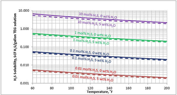
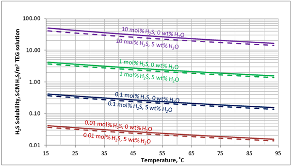
The solubility of acid gases in TEG solution has been the subject of two previous Tips of the Month, (June 2012 and July 2012).  In these instances, the focus was on gas streams with maximum acid gas partial pressure of 100 psia (690 kPa) and TEG concentrations of 95 and 100 wt%.   This is typical for dehydration of sour gas streams.

This month, the focus shifts to the case where the gas is pure CO₂, with partial pressures (and system pressures) ranging up to 800 psia (5 500 kPa), and pure TEG.  These conditions approximate the dehydration of high-CO₂ content gases in a CO₂ enhanced oil recovery project, or perhaps, CO₂ from an industrial source that is to be compressed, transported and sequestered.

Two algorithms have been developed to predict the CO₂ solubility in pure TEG.  One algorithm uses the same format as the Mamrosh-Fisher-Matthews [1] Solubility Model presented in the June 2012 and July 2012 Tips of the Month.  In order to improve the correlation for pure CO₂ and TEG, the equation parameters (A through D) were regressed using data extracted from Figure 20-76 of the GPSA Engineering Data Book [2].  The equation and new parameters are presented below.

In the second algorithm, we propose a 6-parameter empirical equation, which is also regressed from the GPSA Figure 20-76 [2].

Mamrosh-Fisher-Matthews Solubility Model MODIFIED:

The original Mamrosh et al. [1] model, was first applied to data extracted from GPSA Figure 20-76 [2].  Average Absolute Percentage Deviation (AAPD) was greater than 6.5% and the Maximum Absolute Percentage Difference for the data set exceeded 34%.  To improve accuracy, a multi-parameter regression was performed using data from Figure 20-76.  The new values for Parameters A, B, and D (C was set to zero and the original value of E was used) are presented in Table 1 below.

Where:

P is the absolute pressure, psia (kPa(a))

T is the absolute temperature, °R (K)

x_i is the mole fraction of the acid gas in the liquid phase

y_i is the mole fraction of acid gas in the vapor phase

Note that the mole fraction of water in the liquid (  is zero (pure TEG), so parameter “C” has been set to zero.

Table 1. MODIFIED Parameters for Mamrosh et al. model [1]

Accuracy of MODIFIED Mamrosh-Fisher-Matthews Solubility Model:

The accuracy of the MODIFIED Mamrosh et al. [1] model was evaluated against the data extracted from Figure 20-76 of Gas Processors Suppliers Association Engineering Data Book, 12^th Edition [2].  The summary of our evaluation results is shown in Table 2.

Table 2. Summary of error analysis for MODIFIED Mamrosh et al. model

Where:

N = Number of data points

x_i  = mole fraction of acid gas in the liquid phase

Figure 1 presents the data extracted from GPSA Figure 20-76  [2]  for the solubility of pure CO₂ in 100% TEG, and the predicted values from the MODIFIED Mamrosh et al. equation.  GPSA data points are denoted as symbols: Equation results are shown as solid lines.

Overall the accuracy is very good.  At 15 psia, the error looks significant, and the absolute percentage deviation is as high as 10%. However; the actual solubility is small, so the magnitude of the error in physical terms is insignificant.

Proposed CO₂ Solubility Model:

A 6-parameter empirical model was developed by regression of the data extracted from GPSA Figure 20-76  [2].  The general form of the equation is presented as Equation (2) and the values for the six parameters are provided in Table 3.  The model is suitable only for pure CO₂ and 100% TEG.

Figure 1 (FPS). Solubility of pure CO₂ in 100% TEG – GPSA Fig. 20-76 versus MODIFIED Mamrosh et al. Model

NOTE:  Data points from GPSA Fig. 20-76 [2] denoted by symbols: Equation is denoted by solid lines

Figure 1 (SI). Predicted solubility of pure CO₂ in 100% TEG – by MODIFIED Mamrosh et al. Model

Table 2.  Parameters for Moshfeghian model for pure CO₂ in 100% TEG

Accuracy of the Proposed Solubility Model:

The accuracy of the proposed model was evaluated against the data extracted from Figure 20-76 of Gas Processors Suppliers Association Engineering Data Book, 12^th Edition [2]. The summary of our evaluation results is shown in Table 3.

Table 3. Summary of error analysis for Moshfeghian model.

Where AAPD and MAPD are as defined above.

Figure 2 presents the data extracted from GPSA Figure 20-76  [2] for the solubility of pure CO₂ in 100% TEG, and the predicted values from the proposed Model.  GPSA data points are denoted as symbols: Equation results are shown as solid lines.  Also included in Figure 2 are nine data points from GPA Technical Publication TP-9 [3].  These data points are actual values measured for pure CO₂ and 100% TEG at three pressures. Note the TP-9 data were not used in the regression process.

The accuracy of the proposed Model is slightly better than the MODIFIED Mamrosh et al. model.  Average and Maximum Absolute Percentage Deviations are both reduced.  As with the MODIFIED Mamrosh et al. model, the greatest percentage error corresponds to the low pressure case (15 psia or 104 kPa) where the solubility is very small, so the actual deviation is likely insignificant for most engineering calculations.

Figure 3 presents the selected data from GPA RR 183 [4] for the solubility of pure CO₂ in 100% TEG, and the predicted values from the Modified Mamrosh et al. Model and the Proposed Model. These GPA data were not used in regressing either of the two models parameters.

Figure 2 (FPS)  Solubility of pure CO₂ in 100% TEG – GPSA Fig. 20-76 versus the proposed model

NOTES:     Data points extracted from GPSA Fig. 20-76 [2] denoted by symbols: Equation is denoted by solid lines

Large Black symbols and solid lines denote data from GPA TP9 [3]

Figure 2 (SI)  Predicted solubility of pure CO₂ in 100% TEG by the proposed Model

Figure 3.  Comparison of the predicted solubility of pure CO₂ in 100% TEG at 72.5 psia (500 kPaa) with the GPA RR 183 experimental data [4]

Conclusions:

Two new algorithms have been developed to predict the solubility of pure CO₂ in 100% TEG.  Both algorithms were developed by regressing data extracted from Figure 20-76 of the Gas Processors Suppliers Association Engineering Data Books [2]. It should be noted that the Figures in GPSA are attributed to Ed Wichert, Sogapro Engineering with all rights reserved.

The first algorithm is a Modified form of the Mamrosh et al. model [1].  The original model was presented and evaluated for CO₂ concentrations of up to 10 mole percent in the June and July 2012 Tips of the Month. However, model predictions for pure CO₂ and 100% TEG produced an average absolute percentage deviation (AAPD) of more than 6.5%, and a Maximum Absolute Percent Deviation (MAPD) of more than 34% compared with data extracted from Figure 20-76 of the GPSA Engineering Data book [2]. To improve accuracy, the equation parameters were regressed with data points extracted from Figure 20-76.  The Modified Mamrosh et al. model more accurately reproduces the curves in Figure 20-76, with an AAPD of 1.85% and MAPD of 10.1%.

The second algorithm, the proposed Model, uses a different form of the equation.  The six parameter model was also tuned to match data from GPSA Figure 20-76 [2].  The resulting AAPD is 1.50%, and the MAPD is 7.14% compared to Figure 20-76.

To learn more about similar cases and how to minimize operational problems, we suggest attending our G40 (Process/Facility Fundamentals), G4 (Gas Conditioning and Processing), P81 (CO₂ Surface Facilities), and PF4 (Oil Production and Processing Facilities) courses.

John M. Campbell Consulting (JMCC) offers consulting expertise on this subject and many others. For more information about the services JMCC provides, visit our website at www.jmcampbellconsulting.com, or email us at consulting@jmcampbell.com.

By: Wes H. Wright  &  Dr. Mahmood Moshfeghian 

Reference:

1. Mamrosh, D., Fisher, K. and J. Matthews, “Preparing solubility data for use by the gas processing industry:  Updating Key Resources,” Presented at 91^st Gas Processors Association National Convention, New Orleans, Louisiana, USA, April 15-18, 2012.
2. Gas Processors Suppliers Association; “ENGINEERING DATA BOOK” Twelfth Edition – FPS; Tulsa, Oklahoma, USA, 2004.
3. Takahashi, S., Kobayashi, R., “The water content and the solubility of C0₂ in equilibrium with DEG-Water and TEG-Water solutions at feasible absorption conditions,” GPA Technical Publication TP-9, Gas Processors Association, Tulsa, Oklahoma, USA, 1982.
4. Davis, P.M., et al., “The impact of sulfur species on glycol dehydration – Study of the solubility of certain gases and gas mixtures in glycol solutions at the elevated pressures and temperatures,” GPA Research Report 183 (GPA RR 183), Gas Processors Association, Tulsa, Oklahoma, USA, 2002.